10 minutes to Mars DataFrame#
This is a short introduction to Mars DataFrame which is originated from 10 minutes to pandas.
Customarily, we import as follows:
In [1]: import mars

In [2]: import mars.tensor as mt

In [3]: import mars.dataframe as md
Now create a new default session.
In [4]: mars.new_session()
Out[4]: <mars.session.SyncSession at 0x7fdaa4dc1350>
Object creation#
Creating a Series by passing a list of values, letting it create
a default integer index:
In [5]: s = md.Series([1, 3, 5, mt.nan, 6, 8])

In [6]: s.execute()
Out[6]:
0    1.0
1    3.0
2    5.0
3    NaN
4    6.0
5    8.0
dtype: float64
Creating a DataFrame by passing a Mars tensor, with a datetime index
and labeled columns:
In [7]: dates = md.date_range('20130101', periods=6)

In [8]: dates.execute()
Out[8]:
DatetimeIndex(['2013-01-01', '2013-01-02', '2013-01-03', '2013-01-04',
               '2013-01-05', '2013-01-06'],
              dtype='datetime64[ns]', freq='D')

In [9]: df = md.DataFrame(mt.random.randn(6, 4), index=dates, columns=list('ABCD'))

In [10]: df.execute()
Out[10]:
                   A         B         C         D
2013-01-01 -0.416710  0.321854 -0.271996 -2.354697
2013-01-02  0.410208 -0.685989  0.768800  0.199559
2013-01-03  0.814180 -0.133260 -0.630355  0.311276
2013-01-04  0.384856  0.407550  0.589734  0.991019
2013-01-05 -0.817808 -0.710146  0.017860  0.369687
2013-01-06 -0.048851 -1.008527 -1.209015  2.052612
Creating a DataFrame by passing a dict of objects that can be converted to series-like.
In [11]: df2 = md.DataFrame({'A': 1.,
   ....:                     'B': md.Timestamp('20130102'),
   ....:                     'C': md.Series(1, index=list(range(4)), dtype='float32'),
   ....:                     'D': mt.array([3] * 4, dtype='int32'),
   ....:                     'E': 'foo'})
   ....:

In [12]: df2.execute()
Out[12]:
     A          B    C  D    E
0  1.0 2013-01-02  1.0  3  foo
1  1.0 2013-01-02  1.0  3  foo
2  1.0 2013-01-02  1.0  3  foo
3  1.0 2013-01-02  1.0  3  foo
The columns of the resulting DataFrame have different dtypes.
In [13]: df2.dtypes
Out[13]:
A           float64
B    datetime64[ns]
C           float32
D             int32
E            object
dtype: object
Viewing data#
Here is how to view the top and bottom rows of the frame:
In [14]: df.head().execute()
Out[14]:
                   A         B         C         D
2013-01-01 -0.416710  0.321854 -0.271996 -2.354697
2013-01-02  0.410208 -0.685989  0.768800  0.199559
2013-01-03  0.814180 -0.133260 -0.630355  0.311276
2013-01-04  0.384856  0.407550  0.589734  0.991019
2013-01-05 -0.817808 -0.710146  0.017860  0.369687

In [15]: df.tail(3).execute()
Out[15]:
                   A         B         C         D
2013-01-04  0.384856  0.407550  0.589734  0.991019
2013-01-05 -0.817808 -0.710146  0.017860  0.369687
2013-01-06 -0.048851 -1.008527 -1.209015  2.052612
Display the index, columns:
In [16]: df.index.execute()
Out[16]:
DatetimeIndex(['2013-01-01', '2013-01-02', '2013-01-03', '2013-01-04',
               '2013-01-05', '2013-01-06'],
              dtype='datetime64[ns]', freq='D')

In [17]: df.columns.execute()
Out[17]: Index(['A', 'B', 'C', 'D'], dtype='object')
DataFrame.to_tensor() gives a Mars tensor representation of the underlying data.
Note that this can be an expensive operation when your DataFrame has
columns with different data types, which comes down to a fundamental difference
between DataFrame and tensor: tensors have one dtype for the entire tensor,
while DataFrames have one dtype per column. When you call
DataFrame.to_tensor(), Mars DataFrame will find the tensor dtype that can hold all
of the dtypes in the DataFrame. This may end up being object, which requires
casting every value to a Python object.
For df, our DataFrame of all floating-point values,
DataFrame.to_tensor() is fast and doesn’t require copying data.
In [18]: df.to_tensor().execute()
Out[18]:
array([[-0.41670981,  0.32185361, -0.27199631, -2.35469749],
       [ 0.41020753, -0.68598949,  0.76879962,  0.19955858],
       [ 0.81418015, -0.1332603 , -0.63035469,  0.31127637],
       [ 0.38485578,  0.40754961,  0.58973367,  0.99101887],
       [-0.81780828, -0.71014551,  0.01785988,  0.36968717],
       [-0.04885068, -1.00852687, -1.20901478,  2.05261237]])
For df2, the DataFrame with multiple dtypes,
DataFrame.to_tensor() is relatively expensive.
In [19]: df2.to_tensor().execute()
Out[19]:
array([[1.0, Timestamp('2013-01-02 00:00:00'), 1.0, 3, 'foo'],
       [1.0, Timestamp('2013-01-02 00:00:00'), 1.0, 3, 'foo'],
       [1.0, Timestamp('2013-01-02 00:00:00'), 1.0, 3, 'foo'],
       [1.0, Timestamp('2013-01-02 00:00:00'), 1.0, 3, 'foo']],
      dtype=object)
Note
DataFrame.to_tensor() does not include the index or column
labels in the output.
describe() shows a quick statistic summary of your data:
In [20]: df.describe().execute()
Out[20]:
              A         B         C         D
count  6.000000  6.000000  6.000000  6.000000
mean   0.054312 -0.301420 -0.122495  0.261576
std    0.601069  0.588954  0.745945  1.456214
min   -0.817808 -1.008527 -1.209015 -2.354697
25%   -0.324745 -0.704107 -0.540765  0.227488
50%    0.168003 -0.409625 -0.127068  0.340482
75%    0.403870  0.208075  0.446765  0.835686
max    0.814180  0.407550  0.768800  2.052612
Sorting by an axis:
In [21]: df.sort_index(axis=1, ascending=False).execute()
Out[21]:
                   D         C         B         A
2013-01-01 -2.354697 -0.271996  0.321854 -0.416710
2013-01-02  0.199559  0.768800 -0.685989  0.410208
2013-01-03  0.311276 -0.630355 -0.133260  0.814180
2013-01-04  0.991019  0.589734  0.407550  0.384856
2013-01-05  0.369687  0.017860 -0.710146 -0.817808
2013-01-06  2.052612 -1.209015 -1.008527 -0.048851
Sorting by values:
In [22]: df.sort_values(by='B').execute()
Out[22]:
                   A         B         C         D
2013-01-06 -0.048851 -1.008527 -1.209015  2.052612
2013-01-05 -0.817808 -0.710146  0.017860  0.369687
2013-01-02  0.410208 -0.685989  0.768800  0.199559
2013-01-03  0.814180 -0.133260 -0.630355  0.311276
2013-01-01 -0.416710  0.321854 -0.271996 -2.354697
2013-01-04  0.384856  0.407550  0.589734  0.991019
Selection#
Note
While standard Python / Numpy expressions for selecting and setting are
intuitive and come in handy for interactive work, for production code, we
recommend the optimized DataFrame data access methods, .at, .iat,
.loc and .iloc.
Getting#
Selecting a single column, which yields a Series,
equivalent to df.A:
In [23]: df['A'].execute()
Out[23]:
2013-01-01   -0.416710
2013-01-02    0.410208
2013-01-03    0.814180
2013-01-04    0.384856
2013-01-05   -0.817808
2013-01-06   -0.048851
Freq: D, Name: A, dtype: float64
Selecting via [], which slices the rows.
In [24]: df[0:3].execute()
Out[24]:
                   A         B         C         D
2013-01-01 -0.416710  0.321854 -0.271996 -2.354697
2013-01-02  0.410208 -0.685989  0.768800  0.199559
2013-01-03  0.814180 -0.133260 -0.630355  0.311276

In [25]: df['20130102':'20130104'].execute()
Out[25]:
                   A         B         C         D
2013-01-02  0.410208 -0.685989  0.768800  0.199559
2013-01-03  0.814180 -0.133260 -0.630355  0.311276
2013-01-04  0.384856  0.407550  0.589734  0.991019
Selection by label#
For getting a cross section using a label:
In [26]: df.loc['20130101'].execute()
Out[26]:
A   -0.416710
B    0.321854
C   -0.271996
D   -2.354697
Name: 2013-01-01 00:00:00, dtype: float64
Selecting on a multi-axis by label:
In [27]: df.loc[:, ['A', 'B']].execute()
Out[27]:
                   A         B
2013-01-01 -0.416710  0.321854
2013-01-02  0.410208 -0.685989
2013-01-03  0.814180 -0.133260
2013-01-04  0.384856  0.407550
2013-01-05 -0.817808 -0.710146
2013-01-06 -0.048851 -1.008527
Showing label slicing, both endpoints are included:
In [28]: df.loc['20130102':'20130104', ['A', 'B']].execute()
Out[28]:
                   A         B
2013-01-02  0.410208 -0.685989
2013-01-03  0.814180 -0.133260
2013-01-04  0.384856  0.407550
Reduction in the dimensions of the returned object:
In [29]: df.loc['20130102', ['A', 'B']].execute()
Out[29]:
A    0.410208
B   -0.685989
Name: 2013-01-02 00:00:00, dtype: float64
For getting a scalar value:
In [30]: df.loc['20130101', 'A'].execute()
Out[30]: -0.4167098089847822
For getting fast access to a scalar (equivalent to the prior method):
In [31]: df.at['20130101', 'A'].execute()
Out[31]: -0.4167098089847822
Selection by position#
Select via the position of the passed integers:
In [32]: df.iloc[3].execute()
Out[32]:
A    0.384856
B    0.407550
C    0.589734
D    0.991019
Name: 2013-01-04 00:00:00, dtype: float64
By integer slices, acting similar to numpy/python:
In [33]: df.iloc[3:5, 0:2].execute()
Out[33]:
                   A         B
2013-01-04  0.384856  0.407550
2013-01-05 -0.817808 -0.710146
By lists of integer position locations, similar to the numpy/python style:
In [34]: df.iloc[[1, 2, 4], [0, 2]].execute()
Out[34]:
                   A         C
2013-01-02  0.410208  0.768800
2013-01-03  0.814180 -0.630355
2013-01-05 -0.817808  0.017860
For slicing rows explicitly:
In [35]: df.iloc[1:3, :].execute()
Out[35]:
                   A         B         C         D
2013-01-02  0.410208 -0.685989  0.768800  0.199559
2013-01-03  0.814180 -0.133260 -0.630355  0.311276
For slicing columns explicitly:
In [36]: df.iloc[:, 1:3].execute()
Out[36]:
                   B         C
2013-01-01  0.321854 -0.271996
2013-01-02 -0.685989  0.768800
2013-01-03 -0.133260 -0.630355
2013-01-04  0.407550  0.589734
2013-01-05 -0.710146  0.017860
2013-01-06 -1.008527 -1.209015
For getting a value explicitly:
In [37]: df.iloc[1, 1].execute()
Out[37]: -0.6859894870967846
For getting fast access to a scalar (equivalent to the prior method):
In [38]: df.iat[1, 1].execute()
Out[38]: -0.6859894870967846
Boolean indexing#
Using a single column’s values to select data.
In [39]: df[df['A'] > 0].execute()
Out[39]:
                   A         B         C         D
2013-01-02  0.410208 -0.685989  0.768800  0.199559
2013-01-03  0.814180 -0.133260 -0.630355  0.311276
2013-01-04  0.384856  0.407550  0.589734  0.991019
Selecting values from a DataFrame where a boolean condition is met.
In [40]: df[df > 0].execute()
Out[40]:
                   A         B         C         D
2013-01-01       NaN  0.321854       NaN       NaN
2013-01-02  0.410208       NaN  0.768800  0.199559
2013-01-03  0.814180       NaN       NaN  0.311276
2013-01-04  0.384856  0.407550  0.589734  0.991019
2013-01-05       NaN       NaN  0.017860  0.369687
2013-01-06       NaN       NaN       NaN  2.052612
Operations#
Stats#
Operations in general exclude missing data.
Performing a descriptive statistic:
In [41]: df.mean().execute()
Out[41]:
A    0.054312
B   -0.301420
C   -0.122495
D    0.261576
dtype: float64
Same operation on the other axis:
In [42]: df.mean(1).execute()
Out[42]:
2013-01-01   -0.680388
2013-01-02    0.173144
2013-01-03    0.090460
2013-01-04    0.593289
2013-01-05   -0.285102
2013-01-06   -0.053445
Freq: D, dtype: float64
Operating with objects that have different dimensionality and need alignment. In addition, Mars DataFrame automatically broadcasts along the specified dimension.
In [43]: s = md.Series([1, 3, 5, mt.nan, 6, 8], index=dates).shift(2)

In [44]: s.execute()
Out[44]:
2013-01-01    NaN
2013-01-02    NaN
2013-01-03    1.0
2013-01-04    3.0
2013-01-05    5.0
2013-01-06    NaN
Freq: D, dtype: float64

In [45]: df.sub(s, axis='index').execute()
Out[45]:
                   A         B         C         D
2013-01-01       NaN       NaN       NaN       NaN
2013-01-02       NaN       NaN       NaN       NaN
2013-01-03 -0.185820 -1.133260 -1.630355 -0.688724
2013-01-04 -2.615144 -2.592450 -2.410266 -2.008981
2013-01-05 -5.817808 -5.710146 -4.982140 -4.630313
2013-01-06       NaN       NaN       NaN       NaN
Apply#
Applying functions to the data:
In [46]: df.apply(lambda x: x.max() - x.min()).execute()
Out[46]:
A    1.631988
B    1.416076
C    1.977814
D    4.407310
dtype: float64
String Methods#
Series is equipped with a set of string processing methods in the str attribute that make it easy to operate on each element of the array, as in the code snippet below. Note that pattern-matching in str generally uses regular expressions by default (and in some cases always uses them). See more at Vectorized String Methods.
In [47]: s = md.Series(['A', 'B', 'C', 'Aaba', 'Baca', mt.nan, 'CABA', 'dog', 'cat'])

In [48]: s.str.lower().execute()
Out[48]:
0       a
1       b
2       c
3    aaba
4    baca
5     NaN
6    caba
7     dog
8     cat
dtype: object
Merge#
Concat#
Mars DataFrame provides various facilities for easily combining together Series and DataFrame objects with various kinds of set logic for the indexes and relational algebra functionality in the case of join / merge-type operations.
Concatenating DataFrame objects together with concat():
In [49]: df = md.DataFrame(mt.random.randn(10, 4))

In [50]: df.execute()
Out[50]:
          0         1         2         3
0 -0.678447 -0.192182 -2.959549 -0.420776
1 -2.126839  0.393159 -0.621325  1.121568
2 -0.110184  0.795873 -0.998999  0.234943
3  0.214486 -1.132880  1.112513 -1.998890
4 -1.274094 -1.028841 -0.888029  1.088271
5  2.316261  0.041220 -1.527053  0.040022
6  0.688549 -0.497187 -0.608511 -0.176353
7  0.800453 -0.181482  0.935812  1.963344
8  1.222970  0.155696  0.287068 -0.009270
9  0.368088  1.712585  0.970078 -0.545003

# break it into pieces
In [51]: pieces = [df[:3], df[3:7], df[7:]]

In [52]: md.concat(pieces).execute()
Out[52]:
          0         1         2         3
0 -0.678447 -0.192182 -2.959549 -0.420776
1 -2.126839  0.393159 -0.621325  1.121568
2 -0.110184  0.795873 -0.998999  0.234943
3  0.214486 -1.132880  1.112513 -1.998890
4 -1.274094 -1.028841 -0.888029  1.088271
5  2.316261  0.041220 -1.527053  0.040022
6  0.688549 -0.497187 -0.608511 -0.176353
7  0.800453 -0.181482  0.935812  1.963344
8  1.222970  0.155696  0.287068 -0.009270
9  0.368088  1.712585  0.970078 -0.545003
Join#
SQL style merges. See the Database style joining section.
In [53]: left = md.DataFrame({'key': ['foo', 'foo'], 'lval': [1, 2]})

In [54]: right = md.DataFrame({'key': ['foo', 'foo'], 'rval': [4, 5]})

In [55]: left.execute()
Out[55]:
   key  lval
0  foo     1
1  foo     2

In [56]: right.execute()
Out[56]:
   key  rval
0  foo     4
1  foo     5

In [57]: md.merge(left, right, on='key').execute()
Out[57]:
   key  lval  rval
0  foo     1     4
1  foo     1     5
2  foo     2     4
3  foo     2     5
Another example that can be given is:
In [58]: left = md.DataFrame({'key': ['foo', 'bar'], 'lval': [1, 2]})

In [59]: right = md.DataFrame({'key': ['foo', 'bar'], 'rval': [4, 5]})

In [60]: left.execute()
Out[60]:
   key  lval
0  foo     1
1  bar     2

In [61]: right.execute()
Out[61]:
   key  rval
0  foo     4
1  bar     5

In [62]: md.merge(left, right, on='key').execute()
Out[62]:
   key  lval  rval
0  foo     1     4
1  bar     2     5
Grouping#
By “group by” we are referring to a process involving one or more of the following steps:
Splitting the data into groups based on some criteria
Applying a function to each group independently
Combining the results into a data structure
In [63]: df = md.DataFrame({'A': ['foo', 'bar', 'foo', 'bar',
   ....:                          'foo', 'bar', 'foo', 'foo'],
   ....:                    'B': ['one', 'one', 'two', 'three',
   ....:                          'two', 'two', 'one', 'three'],
   ....:                    'C': mt.random.randn(8),
   ....:                    'D': mt.random.randn(8)})
   ....:

In [64]: df.execute()
Out[64]:
     A      B         C         D
0  foo    one  0.384298  1.487053
1  bar    one -0.195042 -0.526442
2  foo    two -0.063552  0.830769
3  bar  three -1.109313 -0.202732
4  foo    two -1.733393 -1.051999
5  bar    two -1.177462  0.852137
6  foo    one  2.370690  1.545228
7  foo  three -0.370274 -0.605404
Grouping and then applying the sum() function to the resulting
groups.
In [65]: df.groupby('A').sum().execute()
Out[65]:
            C         D
A
bar -2.481817  0.122964
foo  0.587768  2.205647
Grouping by multiple columns forms a hierarchical index, and again we can apply the sum function.
In [66]: df.groupby(['A', 'B']).sum().execute()
Out[66]:
                  C         D
A   B
bar one   -0.195042 -0.526442
    three -1.109313 -0.202732
    two   -1.177462  0.852137
foo one    2.754989  3.032281
    three -0.370274 -0.605404
    two   -1.796946 -0.221229
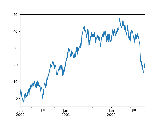
Plotting#
We use the standard convention for referencing the matplotlib API:
In [67]: import matplotlib.pyplot as plt

In [68]: plt.close('all')
In [69]: ts = md.Series(mt.random.randn(1000),
   ....:                index=md.date_range('1/1/2000', periods=1000))
   ....:

In [70]: ts = ts.cumsum()

In [71]: ts.plot()
Out[71]: <AxesSubplot:>
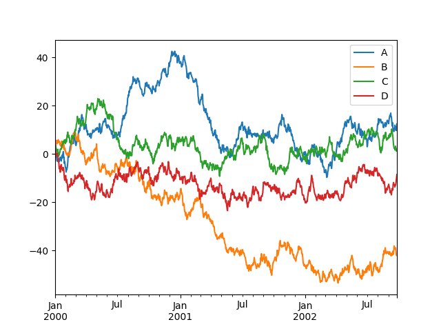
On a DataFrame, the plot() method is a convenience to plot all
of the columns with labels:
In [72]: df = md.DataFrame(mt.random.randn(1000, 4), index=ts.index,
   ....:                   columns=['A', 'B', 'C', 'D'])
   ....:

In [73]: df = df.cumsum()

In [74]: plt.figure()
Out[74]: <Figure size 640x480 with 0 Axes>

In [75]: df.plot()
Out[75]: <AxesSubplot:>

In [76]: plt.legend(loc='best')
Out[76]: <matplotlib.legend.Legend at 0x7fdaa30c7b10>
Getting data in/out#
CSV#
In [77]: df.to_csv('foo.csv').execute()
Out[77]:
Empty DataFrame
Columns: []
Index: []
In [78]: md.read_csv('foo.csv').execute()
Out[78]:
     Unnamed: 0          A          B         C          D
0    2000-01-01  -0.815779   2.099609  0.253410   0.699144
1    2000-01-02  -0.641542   1.014031  1.245225   1.206247
2    2000-01-03   0.886832   3.250385  3.253800   0.412609
3    2000-01-04   0.009398   3.940673  1.910684  -0.079965
4    2000-01-05  -1.064446   5.606098  1.717487  -0.734112
..          ...        ...        ...       ...        ...
995  2002-09-22  11.299699 -38.935741  3.165396 -12.986270
996  2002-09-23   9.768708 -40.099842  2.179037 -12.262168
997  2002-09-24   9.648603 -41.625615  1.890619 -11.113398
998  2002-09-25  10.508900 -42.137707  1.088086  -9.823462
999  2002-09-26  12.386935 -42.059727  1.967928  -8.619892

[1000 rows x 5 columns]