10 分钟入门 Mars DataFrame
本页面是一个对 Mars DataFrame 的简短介绍,内容修改自 10 分钟入门 pandas 。
如果没有说明,我们默认导入下面的包:
In [1]: import mars.tensor as mt

In [2]: import mars.dataframe as md
创建对象
通过传入一个包含值的 list 来创建 Series 实例,并使用默认的整数索引:
In [3]: s = md.Series([1, 3, 5, mt.nan, 6, 8])

In [4]: s.execute()
Out[4]:
0    1.0
1    3.0
2    5.0
3    NaN
4    6.0
5    8.0
dtype: float64
通过一个 Mars Tensor 来创建 DataFrame 实例,并使用时间日期索引和列标签:
In [5]: dates = md.date_range('20130101', periods=6)

In [6]: dates.execute()
Out[6]:
DatetimeIndex(['2013-01-01', '2013-01-02', '2013-01-03', '2013-01-04',
               '2013-01-05', '2013-01-06'],
              dtype='datetime64[ns]', freq='D')

In [7]: df = md.DataFrame(mt.random.randn(6, 4), index=dates, columns=list('ABCD'))

In [8]: df.execute()
Out[8]:
                   A         B         C         D
2013-01-01  1.275796 -1.527831  0.241654 -0.030682
2013-01-02  0.711151  1.069304 -1.812371  0.833372
2013-01-03 -0.954764 -1.395025 -0.020674 -0.913194
2013-01-04  0.569331 -0.090853  0.686371 -0.601624
2013-01-05 -0.209088  0.637392  0.735079  1.898381
2013-01-06  0.546883 -0.985907 -0.295954 -0.167879
通过值可转换为序列的字典来创建 DataFrame 实例:
In [9]: df2 = md.DataFrame({'A': 1.,
   ...:                     'B': md.Timestamp('20130102'),
   ...:                     'C': md.Series(1, index=list(range(4)), dtype='float32'),
   ...:                     'D': mt.array([3] * 4, dtype='int32'),
   ...:                     'E': 'foo'})
   ...:

In [10]: df2.execute()
Out[10]:
     A          B    C  D    E
0  1.0 2013-01-02  1.0  3  foo
1  1.0 2013-01-02  1.0  3  foo
2  1.0 2013-01-02  1.0  3  foo
3  1.0 2013-01-02  1.0  3  foo
最终生成的 DataFrame 中,每列的类型均不相同。
In [11]: df2.dtypes
Out[11]:
A           float64
B    datetime64[ns]
C           float32
D             int32
E            object
dtype: object
查看数据
下面是显示 DataFrame 中开头和结尾若干行的方法:
In [12]: df.head().execute()
Out[12]:
                   A         B         C         D
2013-01-01  1.275796 -1.527831  0.241654 -0.030682
2013-01-02  0.711151  1.069304 -1.812371  0.833372
2013-01-03 -0.954764 -1.395025 -0.020674 -0.913194
2013-01-04  0.569331 -0.090853  0.686371 -0.601624
2013-01-05 -0.209088  0.637392  0.735079  1.898381

In [13]: df.tail(3).execute()
Out[13]:
                   A         B         C         D
2013-01-04  0.569331 -0.090853  0.686371 -0.601624
2013-01-05 -0.209088  0.637392  0.735079  1.898381
2013-01-06  0.546883 -0.985907 -0.295954 -0.167879
显示索引和列:
In [14]: df.index.execute()
Out[14]:
DatetimeIndex(['2013-01-01', '2013-01-02', '2013-01-03', '2013-01-04',
               '2013-01-05', '2013-01-06'],
              dtype='datetime64[ns]', freq='D')

In [15]: df.columns.execute()
Out[15]: Index(['A', 'B', 'C', 'D'], dtype='object')
DataFrame.to_tensor() 将 DataFrame 中的数据转换为 Mars Tensor 表示。注意当 DataFrame 中的列类型不同时,该操作可能代价很高。这也揭示了 DataFrame 和 Tensor 之间一项最基本的差异:在 Tensor 中,对于整个 Tensor 对象只有一个 dtype,但 DataFrame 对每列都有一个 dtype。当调用 DataFrame.to_tensor() 时,Mars DataFrame 将会找出一个可存储 DataFrame 中 所有 对象的 dtype,这可能是一个 object,并将导致 DataFrame 中的每个值都被转换为一个 Python 对象。
在上面的 df 对象中,DataFrame 实例中的值均为浮点数,因而 DataFrame.to_tensor() 执行速度会很快,且不需要数据复制。
In [16]: df.to_tensor().execute()
Out[16]:
array([[ 1.2757958 , -1.52783113,  0.24165425, -0.03068215],
       [ 0.71115076,  1.06930425, -1.81237108,  0.83337183],
       [-0.95476379, -1.39502471, -0.02067401, -0.91319356],
       [ 0.56933053, -0.09085267,  0.68637103, -0.60162407],
       [-0.20908757,  0.63739234,  0.73507933,  1.89838064],
       [ 0.54688311, -0.98590713, -0.29595356, -0.16787889]])
而对于 df2 对象,DataFrame 实例中有不同的数据类型,因而 DataFrame.to_tensor() 执行代价就相对较高了。
In [17]: df2.to_tensor().execute()
Out[17]:
array([[1.0, Timestamp('2013-01-02 00:00:00'), 1.0, 3, 'foo'],
       [1.0, Timestamp('2013-01-02 00:00:00'), 1.0, 3, 'foo'],
       [1.0, Timestamp('2013-01-02 00:00:00'), 1.0, 3, 'foo'],
       [1.0, Timestamp('2013-01-02 00:00:00'), 1.0, 3, 'foo']],
      dtype=object)
注解
DataFrame.to_tensor() 在输出结果中 不保留 索引或列标签。
describe() 将会为你的数据显示一份简单的统计摘要:
In [18]: df.describe().execute()
Out[18]:
              A         B         C         D
count  6.000000  6.000000  6.000000  6.000000
mean   0.323218 -0.382153 -0.077649  0.169729
std    0.785504  1.089409  0.938762  1.034457
min   -0.954764 -1.527831 -1.812371 -0.913194
25%   -0.020095 -1.292745 -0.227134 -0.493188
50%    0.558107 -0.538380  0.110490 -0.099281
75%    0.675696  0.455331  0.575192  0.617358
max    1.275796  1.069304  0.735079  1.898381
按坐标排序:
In [19]: df.sort_index(axis=1, ascending=False).execute()
Out[19]:
                   D         C         B         A
2013-01-01 -0.030682  0.241654 -1.527831  1.275796
2013-01-02  0.833372 -1.812371  1.069304  0.711151
2013-01-03 -0.913194 -0.020674 -1.395025 -0.954764
2013-01-04 -0.601624  0.686371 -0.090853  0.569331
2013-01-05  1.898381  0.735079  0.637392 -0.209088
2013-01-06 -0.167879 -0.295954 -0.985907  0.546883
按值排序:
In [20]: df.sort_values(by='B').execute()
Out[20]:
                   A         B         C         D
2013-01-01  1.275796 -1.527831  0.241654 -0.030682
2013-01-03 -0.954764 -1.395025 -0.020674 -0.913194
2013-01-06  0.546883 -0.985907 -0.295954 -0.167879
2013-01-04  0.569331 -0.090853  0.686371 -0.601624
2013-01-05 -0.209088  0.637392  0.735079  1.898381
2013-01-02  0.711151  1.069304 -1.812371  0.833372
选择数据
注解
尽管在交互式分析场景下,使用标准的 Python / Numpy 表达式选择和设置 DataFrame 数据非常自然且便于使用,但对生产代码,我们推荐使用经过优化的数据访问方法,即 .at、.iat、.loc 和 .iloc。
获取数据
选择一列,将返回一个 Series 实例。这一操作等价于 df.A :
In [21]: df['A'].execute()
Out[21]:
2013-01-01    1.275796
2013-01-02    0.711151
2013-01-03   -0.954764
2013-01-04    0.569331
2013-01-05   -0.209088
2013-01-06    0.546883
Freq: D, Name: A, dtype: float64
通过 [] 选择数据,将在行中选取。
In [22]: df[0:3].execute()
Out[22]:
                   A         B         C         D
2013-01-01  1.275796 -1.527831  0.241654 -0.030682
2013-01-02  0.711151  1.069304 -1.812371  0.833372
2013-01-03 -0.954764 -1.395025 -0.020674 -0.913194

In [23]: df['20130102':'20130104'].execute()
Out[23]:
                   A         B         C         D
2013-01-02  0.711151  1.069304 -1.812371  0.833372
2013-01-03 -0.954764 -1.395025 -0.020674 -0.913194
2013-01-04  0.569331 -0.090853  0.686371 -0.601624
按标签选择数据
通过行标签选择一行数据:
In [24]: df.loc['20130101'].execute()
Out[24]:
A    1.275796
B   -1.527831
C    0.241654
D   -0.030682
Name: 2013-01-01 00:00:00, dtype: float64
在特定坐标上指定标签:
In [25]: df.loc[:, ['A', 'B']].execute()
Out[25]:
                   A         B
2013-01-01  1.275796 -1.527831
2013-01-02  0.711151  1.069304
2013-01-03 -0.954764 -1.395025
2013-01-04  0.569331 -0.090853
2013-01-05 -0.209088  0.637392
2013-01-06  0.546883 -0.985907
在多个坐标上指定标签,带有这些标签的 所有数据 均会被选取:
In [26]: df.loc['20130102':'20130104', ['A', 'B']].execute()
Out[26]:
                   A         B
2013-01-02  0.711151  1.069304
2013-01-03 -0.954764 -1.395025
2013-01-04  0.569331 -0.090853
在特定坐标上降低返回对象的维度:
In [27]: df.loc['20130102', ['A', 'B']].execute()
Out[27]:
A    0.711151
B    1.069304
Name: 2013-01-02 00:00:00, dtype: float64
获得一个常量:
In [28]: df.loc['20130101', 'A'].execute()
Out[28]: 1.275795797291396
快速获取一个常数(和前述方法等价):
In [29]: df.at['20130101', 'A'].execute()
Out[29]: 1.275795797291396
按位置选择
通过传入的整数选择相应位置的数据:
In [30]: df.iloc[3].execute()
Out[30]:
A    0.569331
B   -0.090853
C    0.686371
D   -0.601624
Name: 2013-01-04 00:00:00, dtype: float64
通过整数切片来选择数据,与 Numpy / Python 行为一致:
In [31]: df.iloc[3:5, 0:2].execute()
Out[31]:
                   A         B
2013-01-04  0.569331 -0.090853
2013-01-05 -0.209088  0.637392
通过整数列表选择相应位置的数据,与 Numpy / Python 行为一致:
In [32]: df.iloc[[1, 2, 4], [0, 2]].execute()
Out[32]:
                   A         C
2013-01-02  0.711151 -1.812371
2013-01-03 -0.954764 -0.020674
2013-01-05 -0.209088  0.735079
显示对行切片:
In [33]: df.iloc[1:3, :].execute()
Out[33]:
                   A         B         C         D
2013-01-02  0.711151  1.069304 -1.812371  0.833372
2013-01-03 -0.954764 -1.395025 -0.020674 -0.913194
显示对列切片:
In [34]: df.iloc[:, 1:3].execute()
Out[34]:
                   B         C
2013-01-01 -1.527831  0.241654
2013-01-02  1.069304 -1.812371
2013-01-03 -1.395025 -0.020674
2013-01-04 -0.090853  0.686371
2013-01-05  0.637392  0.735079
2013-01-06 -0.985907 -0.295954
显示获取某个位置的常数:
In [35]: df.iloc[1, 1].execute()
Out[35]: 1.0693042509838953
快速获取一个常数(和前述方法等价):
In [36]: df.iat[1, 1].execute()
Out[36]: 1.0693042509838953
布尔索引
使用一行布尔值选择数据:
In [37]: df[df['A'] > 0].execute()
Out[37]:
                   A         B         C         D
2013-01-01  1.275796 -1.527831  0.241654 -0.030682
2013-01-02  0.711151  1.069304 -1.812371  0.833372
2013-01-04  0.569331 -0.090853  0.686371 -0.601624
2013-01-06  0.546883 -0.985907 -0.295954 -0.167879
从 DataFrame 选择满足某个布尔条件的值:
In [38]: df[df > 0].execute()
Out[38]:
                   A         B         C         D
2013-01-01  1.275796       NaN  0.241654       NaN
2013-01-02  0.711151  1.069304       NaN  0.833372
2013-01-03       NaN       NaN       NaN       NaN
2013-01-04  0.569331       NaN  0.686371       NaN
2013-01-05       NaN  0.637392  0.735079  1.898381
2013-01-06  0.546883       NaN       NaN       NaN
数据操作
统计
除缺失值外的常见操作:
计算描述统计值:
In [39]: df.mean().execute()
Out[39]:
A    0.323218
B   -0.382153
C   -0.077649
D    0.169729
dtype: float64
在另一条坐标轴上进行相同的操作:
In [40]: df.mean(1).execute()
Out[40]:
2013-01-01   -0.010266
2013-01-02    0.200364
2013-01-03   -0.820914
2013-01-04    0.140806
2013-01-05    0.765441
2013-01-06   -0.225714
Freq: D, dtype: float64
在维度不同的对象上进行操作,这需要进行对齐。此外,Mars DataFrame 会自动在给定的坐标轴上对数据进行广播操作。
In [41]: s = md.Series([1, 3, 5, mt.nan, 6, 8], index=dates).shift(2)

In [42]: s.execute()
Out[42]:
2013-01-01    NaN
2013-01-02    NaN
2013-01-03    1.0
2013-01-04    3.0
2013-01-05    5.0
2013-01-06    NaN
Freq: D, dtype: float64

In [43]: df.sub(s, axis='index').execute()
Out[43]:
                   A         B         C         D
2013-01-01       NaN       NaN       NaN       NaN
2013-01-02       NaN       NaN       NaN       NaN
2013-01-03 -1.954764 -2.395025 -1.020674 -1.913194
2013-01-04 -2.430669 -3.090853 -2.313629 -3.601624
2013-01-05 -5.209088 -4.362608 -4.264921 -3.101619
2013-01-06       NaN       NaN       NaN       NaN
应用函数
在数据上应用函数:
In [44]: df.apply(lambda x: x.max() - x.min()).execute()
Out[44]:
A    2.230560
B    2.597135
C    2.547450
D    2.811574
dtype: float64
字符串方法
如同下面的例子展示的那样,Series 对象通过 str 属性提供了一系列字符串操作方法以便于操作每一个元素。注意通过 str 进行的模式匹配通常会默认(在某些情形下会一直)用到 正则表达式 。更多的信息可在 向量化字符串方法 中查看。
In [45]: s = md.Series(['A', 'B', 'C', 'Aaba', 'Baca', mt.nan, 'CABA', 'dog', 'cat'])

In [46]: s.str.lower().execute()
Out[46]:
0       a
1       b
2       c
3    aaba
4    baca
5     NaN
6    caba
7     dog
8     cat
dtype: object
数据合并
拼接
Mars DataFrame 提供一系列的方法方便地将 Series 和 DataFrame 对象连接到一起。这些方法基于一系列在索引上的集合逻辑以及关系代数上的功能来实现 Join / 合并这样的操作。
通过 concat(): 拼接 DataFrame 对象:
In [47]: df = md.DataFrame(mt.random.randn(10, 4))

In [48]: df.execute()
Out[48]:
          0         1         2         3
0  0.659598 -0.681777 -0.361253 -0.060405
1 -0.841487 -1.336353  0.751517 -0.509664
2  0.286396  0.973381  0.552076 -1.503819
3 -1.765832  0.750991  0.369950 -0.520721
4 -0.125677  1.395948  0.873103 -0.668297
5 -1.036919 -1.198912  1.114260  1.335443
6  0.553841  0.430796  0.892376  2.124102
7  0.519051 -1.075312  2.623851  0.673538
8  0.622550  0.830736  0.247380 -0.304671
9  0.476587  0.652279 -0.333462  0.592048

# break it into pieces
In [49]: pieces = [df[:3], df[3:7], df[7:]]

In [50]: md.concat(pieces).execute()
Out[50]:
          0         1         2         3
0  0.659598 -0.681777 -0.361253 -0.060405
1 -0.841487 -1.336353  0.751517 -0.509664
2  0.286396  0.973381  0.552076 -1.503819
3 -1.765832  0.750991  0.369950 -0.520721
4 -0.125677  1.395948  0.873103 -0.668297
5 -1.036919 -1.198912  1.114260  1.335443
6  0.553841  0.430796  0.892376  2.124102
7  0.519051 -1.075312  2.623851  0.673538
8  0.622550  0.830736  0.247380 -0.304671
9  0.476587  0.652279 -0.333462  0.592048
Join
SQL 样式的数据合并。参考 Database style joining 章节以获取更多信息。
In [51]: left = md.DataFrame({'key': ['foo', 'foo'], 'lval': [1, 2]})

In [52]: right = md.DataFrame({'key': ['foo', 'foo'], 'rval': [4, 5]})

In [53]: left.execute()
Out[53]:
   key  lval
0  foo     1
1  foo     2

In [54]: right.execute()
Out[54]:
   key  rval
0  foo     4
1  foo     5

In [55]: md.merge(left, right, on='key').execute()
Out[55]:
   key  lval  rval
0  foo     1     4
1  foo     1     5
2  foo     2     4
3  foo     2     5
另一个可供参考的例子如下:
In [56]: left = md.DataFrame({'key': ['foo', 'bar'], 'lval': [1, 2]})

In [57]: right = md.DataFrame({'key': ['foo', 'bar'], 'rval': [4, 5]})

In [58]: left.execute()
Out[58]:
   key  lval
0  foo     1
1  bar     2

In [59]: right.execute()
Out[59]:
   key  rval
0  foo     4
1  bar     5

In [60]: md.merge(left, right, on='key').execute()
Out[60]:
   key  lval  rval
0  foo     1     4
1  bar     2     5
分组
当提到“分组”时,我们指的是下面一个或多个步骤组成的过程:
拆分 :根据某些条件将数据拆分成组
应用函数 :对每一组数据分别应用某个函数
合并 :将结果合并为一组数据
In [61]: df = md.DataFrame({'A': ['foo', 'bar', 'foo', 'bar',
   ....:                          'foo', 'bar', 'foo', 'foo'],
   ....:                    'B': ['one', 'one', 'two', 'three',
   ....:                          'two', 'two', 'one', 'three'],
   ....:                    'C': mt.random.randn(8),
   ....:                    'D': mt.random.randn(8)})
   ....:

In [62]: df.execute()
Out[62]:
     A      B         C         D
0  foo    one  0.704247 -0.423476
1  bar    one  0.138073  0.810828
2  foo    two -0.204015 -0.338593
3  bar  three  0.586154 -0.186483
4  foo    two  0.586651 -0.917937
5  bar    two  0.649538  0.445192
6  foo    one  0.218760  0.079968
7  foo  three  0.194587  0.822140
分组,然后在结果上执行 sum() 函数。
In [63]: df.groupby('A').sum().execute()
Out[63]:
            C         D
A
bar  1.373766  1.069536
foo  1.500230 -0.777898
我们也可以利用多列进行分组,这将形成一个多重索引。在此结果上,我们也可以执行 sum 函数。
In [64]: df.groupby(['A', 'B']).sum().execute()
Out[64]:
                  C         D
A   B
foo one    0.923007 -0.343509
    two    0.382636 -1.256530
    three  0.194587  0.822140
bar one    0.138073  0.810828
    two    0.649538  0.445192
    three  0.586154 -0.186483
绘图
我们使用标准的约定来引用 matplotlib API:
In [65]: import matplotlib.pyplot as plt

In [66]: plt.close('all')
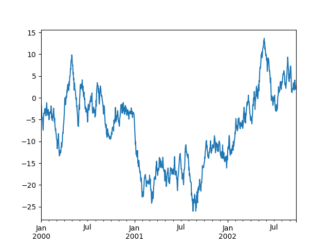
In [67]: ts = md.Series(mt.random.randn(1000),
   ....:                index=md.date_range('1/1/2000', periods=1000))
   ....:

In [68]: ts = ts.cumsum()

In [69]: ts.plot()
Out[69]: <AxesSubplot:>
在 DataFrame 中, plot() 方法可用于方便地绘制带有标签的行数据:
In [70]: df = md.DataFrame(mt.random.randn(1000, 4), index=ts.index,
   ....:                   columns=['A', 'B', 'C', 'D'])
   ....:

In [71]: df = df.cumsum()

In [72]: plt.figure()
Out[72]: <Figure size 640x480 with 0 Axes>

In [73]: df.plot()
Out[73]: <AxesSubplot:>

In [74]: plt.legend(loc='best')
Out[74]: <matplotlib.legend.Legend at 0x7f58081c6810>

读取和写入数据
CSV
In [75]: df.to_csv('foo.csv').execute()
Out[75]:
Empty DataFrame
Columns: []
Index: []
In [76]: md.read_csv('foo.csv').execute()
Out[76]:
     Unnamed: 0         A          B          C         D
0    2000-01-01  0.525186   0.426962  -0.273423  0.385710
1    2000-01-02 -0.290646  -0.913541  -3.042747  0.499835
2    2000-01-03  0.447457  -1.295757  -4.121023 -0.593219
3    2000-01-04  0.348950  -2.322628  -4.796107  0.276122
4    2000-01-05  0.258872  -1.178265  -4.686592 -0.069901
..          ...       ...        ...        ...       ...
995  2002-09-22  7.574156  15.081313 -17.091432 -5.817799
996  2002-09-23  8.099651  14.799730 -16.416023 -6.090026
997  2002-09-24  5.308885  14.602450 -14.787049 -5.086516
998  2002-09-25  6.054512  15.575162 -16.338427 -6.956904
999  2002-09-26  5.616608  16.325124 -17.027597 -6.531918

[1000 rows x 5 columns]