10 minutes to Mars DataFrame
This is a short introduction to Mars DataFrame which is originated from 10 minutes to pandas.
Customarily, we import as follows:
In [1]: import mars

In [2]: import mars.tensor as mt

In [3]: import mars.dataframe as md
Now create a new default session.
In [4]: mars.new_session()
Out[4]: <mars.deploy.oscar.session.SyncSession at 0x7efb742dd350>
Object creation
Creating a Series by passing a list of values, letting it create
a default integer index:
In [5]: s = md.Series([1, 3, 5, mt.nan, 6, 8])

In [6]: s.execute()
Out[6]:
0    1.0
1    3.0
2    5.0
3    NaN
4    6.0
5    8.0
dtype: float64
Creating a DataFrame by passing a Mars tensor, with a datetime index
and labeled columns:
In [7]: dates = md.date_range('20130101', periods=6)

In [8]: dates.execute()
Out[8]:
DatetimeIndex(['2013-01-01', '2013-01-02', '2013-01-03', '2013-01-04',
               '2013-01-05', '2013-01-06'],
              dtype='datetime64[ns]', freq='D')

In [9]: df = md.DataFrame(mt.random.randn(6, 4), index=dates, columns=list('ABCD'))

In [10]: df.execute()
Out[10]:
                   A         B         C         D
2013-01-01 -0.126299  1.264629  1.756465 -0.785511
2013-01-02  0.992830  0.394886 -0.808420 -0.681974
2013-01-03  1.083691 -0.113957  1.493871  2.664410
2013-01-04 -1.157074 -0.158821 -2.012260  1.202826
2013-01-05 -1.744805 -0.966685  0.935808  0.615988
2013-01-06  0.061212 -0.330839 -0.468423 -0.927937
Creating a DataFrame by passing a dict of objects that can be converted to series-like.
In [11]: df2 = md.DataFrame({'A': 1.,
   ....:                     'B': md.Timestamp('20130102'),
   ....:                     'C': md.Series(1, index=list(range(4)), dtype='float32'),
   ....:                     'D': mt.array([3] * 4, dtype='int32'),
   ....:                     'E': 'foo'})
   ....:

In [12]: df2.execute()
Out[12]:
     A          B    C  D    E
0  1.0 2013-01-02  1.0  3  foo
1  1.0 2013-01-02  1.0  3  foo
2  1.0 2013-01-02  1.0  3  foo
3  1.0 2013-01-02  1.0  3  foo
The columns of the resulting DataFrame have different dtypes.
In [13]: df2.dtypes
Out[13]:
A           float64
B    datetime64[ns]
C           float32
D             int32
E            object
dtype: object
Viewing data
Here is how to view the top and bottom rows of the frame:
In [14]: df.head().execute()
Out[14]:
                   A         B         C         D
2013-01-01 -0.126299  1.264629  1.756465 -0.785511
2013-01-02  0.992830  0.394886 -0.808420 -0.681974
2013-01-03  1.083691 -0.113957  1.493871  2.664410
2013-01-04 -1.157074 -0.158821 -2.012260  1.202826
2013-01-05 -1.744805 -0.966685  0.935808  0.615988

In [15]: df.tail(3).execute()
Out[15]:
                   A         B         C         D
2013-01-04 -1.157074 -0.158821 -2.012260  1.202826
2013-01-05 -1.744805 -0.966685  0.935808  0.615988
2013-01-06  0.061212 -0.330839 -0.468423 -0.927937
Display the index, columns:
In [16]: df.index.execute()
Out[16]:
DatetimeIndex(['2013-01-01', '2013-01-02', '2013-01-03', '2013-01-04',
               '2013-01-05', '2013-01-06'],
              dtype='datetime64[ns]', freq='D')

In [17]: df.columns.execute()
Out[17]: Index(['A', 'B', 'C', 'D'], dtype='object')
DataFrame.to_tensor() gives a Mars tensor representation of the underlying data.
Note that this can be an expensive operation when your DataFrame has
columns with different data types, which comes down to a fundamental difference
between DataFrame and tensor: tensors have one dtype for the entire tensor,
while DataFrames have one dtype per column. When you call
DataFrame.to_tensor(), Mars DataFrame will find the tensor dtype that can hold all
of the dtypes in the DataFrame. This may end up being object, which requires
casting every value to a Python object.
For df, our DataFrame of all floating-point values,
DataFrame.to_tensor() is fast and doesn’t require copying data.
In [18]: df.to_tensor().execute()
Out[18]:
array([[-0.12629922,  1.26462895,  1.75646523, -0.7855111 ],
       [ 0.99283028,  0.39488617, -0.80842043, -0.6819743 ],
       [ 1.08369102, -0.11395731,  1.49387063,  2.66440973],
       [-1.1570743 , -0.15882131, -2.01225998,  1.20282606],
       [-1.74480452, -0.96668512,  0.93580838,  0.61598812],
       [ 0.06121177, -0.33083876, -0.46842291, -0.92793697]])
For df2, the DataFrame with multiple dtypes,
DataFrame.to_tensor() is relatively expensive.
In [19]: df2.to_tensor().execute()
Out[19]:
array([[1.0, Timestamp('2013-01-02 00:00:00'), 1.0, 3, 'foo'],
       [1.0, Timestamp('2013-01-02 00:00:00'), 1.0, 3, 'foo'],
       [1.0, Timestamp('2013-01-02 00:00:00'), 1.0, 3, 'foo'],
       [1.0, Timestamp('2013-01-02 00:00:00'), 1.0, 3, 'foo']],
      dtype=object)
Note
DataFrame.to_tensor() does not include the index or column
labels in the output.
describe() shows a quick statistic summary of your data:
In [20]: df.describe().execute()
Out[20]:
              A         B         C         D
count  6.000000  6.000000  6.000000  6.000000
mean  -0.148407  0.014869  0.149507  0.347967
std    1.134091  0.753132  1.481931  1.424220
min   -1.744805 -0.966685 -2.012260 -0.927937
25%   -0.899381 -0.287834 -0.723421 -0.759627
50%   -0.032544 -0.136389  0.233693 -0.032993
75%    0.759926  0.267675  1.354355  1.056117
max    1.083691  1.264629  1.756465  2.664410
Sorting by an axis:
In [21]: df.sort_index(axis=1, ascending=False).execute()
Out[21]:
                   D         C         B         A
2013-01-01 -0.785511  1.756465  1.264629 -0.126299
2013-01-02 -0.681974 -0.808420  0.394886  0.992830
2013-01-03  2.664410  1.493871 -0.113957  1.083691
2013-01-04  1.202826 -2.012260 -0.158821 -1.157074
2013-01-05  0.615988  0.935808 -0.966685 -1.744805
2013-01-06 -0.927937 -0.468423 -0.330839  0.061212
Sorting by values:
In [22]: df.sort_values(by='B').execute()
Out[22]:
                   A         B         C         D
2013-01-05 -1.744805 -0.966685  0.935808  0.615988
2013-01-06  0.061212 -0.330839 -0.468423 -0.927937
2013-01-04 -1.157074 -0.158821 -2.012260  1.202826
2013-01-03  1.083691 -0.113957  1.493871  2.664410
2013-01-02  0.992830  0.394886 -0.808420 -0.681974
2013-01-01 -0.126299  1.264629  1.756465 -0.785511
Selection
Note
While standard Python / Numpy expressions for selecting and setting are
intuitive and come in handy for interactive work, for production code, we
recommend the optimized DataFrame data access methods, .at, .iat,
.loc and .iloc.
Getting
Selecting a single column, which yields a Series,
equivalent to df.A:
In [23]: df['A'].execute()
Out[23]:
2013-01-01   -0.126299
2013-01-02    0.992830
2013-01-03    1.083691
2013-01-04   -1.157074
2013-01-05   -1.744805
2013-01-06    0.061212
Freq: D, Name: A, dtype: float64
Selecting via [], which slices the rows.
In [24]: df[0:3].execute()
Out[24]:
                   A         B         C         D
2013-01-01 -0.126299  1.264629  1.756465 -0.785511
2013-01-02  0.992830  0.394886 -0.808420 -0.681974
2013-01-03  1.083691 -0.113957  1.493871  2.664410

In [25]: df['20130102':'20130104'].execute()
Out[25]:
                   A         B         C         D
2013-01-02  0.992830  0.394886 -0.808420 -0.681974
2013-01-03  1.083691 -0.113957  1.493871  2.664410
2013-01-04 -1.157074 -0.158821 -2.012260  1.202826
Selection by label
For getting a cross section using a label:
In [26]: df.loc['20130101'].execute()
Out[26]:
A   -0.126299
B    1.264629
C    1.756465
D   -0.785511
Name: 2013-01-01 00:00:00, dtype: float64
Selecting on a multi-axis by label:
In [27]: df.loc[:, ['A', 'B']].execute()
Out[27]:
                   A         B
2013-01-01 -0.126299  1.264629
2013-01-02  0.992830  0.394886
2013-01-03  1.083691 -0.113957
2013-01-04 -1.157074 -0.158821
2013-01-05 -1.744805 -0.966685
2013-01-06  0.061212 -0.330839
Showing label slicing, both endpoints are included:
In [28]: df.loc['20130102':'20130104', ['A', 'B']].execute()
Out[28]:
                   A         B
2013-01-02  0.992830  0.394886
2013-01-03  1.083691 -0.113957
2013-01-04 -1.157074 -0.158821
Reduction in the dimensions of the returned object:
In [29]: df.loc['20130102', ['A', 'B']].execute()
Out[29]:
A    0.992830
B    0.394886
Name: 2013-01-02 00:00:00, dtype: float64
For getting a scalar value:
In [30]: df.loc['20130101', 'A'].execute()
Out[30]: -0.12629922084962217
For getting fast access to a scalar (equivalent to the prior method):
In [31]: df.at['20130101', 'A'].execute()
Out[31]: -0.12629922084962217
Selection by position
Select via the position of the passed integers:
In [32]: df.iloc[3].execute()
Out[32]:
A   -1.157074
B   -0.158821
C   -2.012260
D    1.202826
Name: 2013-01-04 00:00:00, dtype: float64
By integer slices, acting similar to numpy/python:
In [33]: df.iloc[3:5, 0:2].execute()
Out[33]:
                   A         B
2013-01-04 -1.157074 -0.158821
2013-01-05 -1.744805 -0.966685
By lists of integer position locations, similar to the numpy/python style:
In [34]: df.iloc[[1, 2, 4], [0, 2]].execute()
Out[34]:
                   A         C
2013-01-02  0.992830 -0.808420
2013-01-03  1.083691  1.493871
2013-01-05 -1.744805  0.935808
For slicing rows explicitly:
In [35]: df.iloc[1:3, :].execute()
Out[35]:
                   A         B         C         D
2013-01-02  0.992830  0.394886 -0.808420 -0.681974
2013-01-03  1.083691 -0.113957  1.493871  2.664410
For slicing columns explicitly:
In [36]: df.iloc[:, 1:3].execute()
Out[36]:
                   B         C
2013-01-01  1.264629  1.756465
2013-01-02  0.394886 -0.808420
2013-01-03 -0.113957  1.493871
2013-01-04 -0.158821 -2.012260
2013-01-05 -0.966685  0.935808
2013-01-06 -0.330839 -0.468423
For getting a value explicitly:
In [37]: df.iloc[1, 1].execute()
Out[37]: 0.39488617338325527
For getting fast access to a scalar (equivalent to the prior method):
In [38]: df.iat[1, 1].execute()
Out[38]: 0.39488617338325527
Boolean indexing
Using a single column’s values to select data.
In [39]: df[df['A'] > 0].execute()
Out[39]:
                   A         B         C         D
2013-01-02  0.992830  0.394886 -0.808420 -0.681974
2013-01-03  1.083691 -0.113957  1.493871  2.664410
2013-01-06  0.061212 -0.330839 -0.468423 -0.927937
Selecting values from a DataFrame where a boolean condition is met.
In [40]: df[df > 0].execute()
Out[40]:
                   A         B         C         D
2013-01-01       NaN  1.264629  1.756465       NaN
2013-01-02  0.992830  0.394886       NaN       NaN
2013-01-03  1.083691       NaN  1.493871  2.664410
2013-01-04       NaN       NaN       NaN  1.202826
2013-01-05       NaN       NaN  0.935808  0.615988
2013-01-06  0.061212       NaN       NaN       NaN
Operations
Stats
Operations in general exclude missing data.
Performing a descriptive statistic:
In [41]: df.mean().execute()
Out[41]:
A   -0.148407
B    0.014869
C    0.149507
D    0.347967
dtype: float64
Same operation on the other axis:
In [42]: df.mean(1).execute()
Out[42]:
2013-01-01    0.527321
2013-01-02   -0.025670
2013-01-03    1.282004
2013-01-04   -0.531332
2013-01-05   -0.289923
2013-01-06   -0.416497
Freq: D, dtype: float64
Operating with objects that have different dimensionality and need alignment. In addition, Mars DataFrame automatically broadcasts along the specified dimension.
In [43]: s = md.Series([1, 3, 5, mt.nan, 6, 8], index=dates).shift(2)

In [44]: s.execute()
Out[44]:
2013-01-01    NaN
2013-01-02    NaN
2013-01-03    1.0
2013-01-04    3.0
2013-01-05    5.0
2013-01-06    NaN
Freq: D, dtype: float64

In [45]: df.sub(s, axis='index').execute()
Out[45]:
                   A         B         C         D
2013-01-01       NaN       NaN       NaN       NaN
2013-01-02       NaN       NaN       NaN       NaN
2013-01-03  0.083691 -1.113957  0.493871  1.664410
2013-01-04 -4.157074 -3.158821 -5.012260 -1.797174
2013-01-05 -6.744805 -5.966685 -4.064192 -4.384012
2013-01-06       NaN       NaN       NaN       NaN
Apply
Applying functions to the data:
In [46]: df.apply(lambda x: x.max() - x.min()).execute()
Out[46]:
A    2.828496
B    2.231314
C    3.768725
D    3.592347
dtype: float64
String Methods
Series is equipped with a set of string processing methods in the str attribute that make it easy to operate on each element of the array, as in the code snippet below. Note that pattern-matching in str generally uses regular expressions by default (and in some cases always uses them). See more at Vectorized String Methods.
In [47]: s = md.Series(['A', 'B', 'C', 'Aaba', 'Baca', mt.nan, 'CABA', 'dog', 'cat'])

In [48]: s.str.lower().execute()
Out[48]:
0       a
1       b
2       c
3    aaba
4    baca
5     NaN
6    caba
7     dog
8     cat
dtype: object
Merge
Concat
Mars DataFrame provides various facilities for easily combining together Series and DataFrame objects with various kinds of set logic for the indexes and relational algebra functionality in the case of join / merge-type operations.
Concatenating DataFrame objects together with concat():
In [49]: df = md.DataFrame(mt.random.randn(10, 4))

In [50]: df.execute()
Out[50]:
          0         1         2         3
0 -0.144211  1.375899  0.118131  0.677074
1  1.051823  1.774792 -0.442876  0.407749
2 -1.470332 -0.744221  1.466971 -1.049013
3 -0.844817 -1.051110 -0.363198  0.064381
4  1.675680 -0.822511 -0.554110  1.400377
5  1.169133 -0.980388 -0.413070  0.541066
6 -0.536081 -1.555884  0.479434  1.405025
7  1.477188  0.869055  1.317190  0.347329
8  0.527675  0.846943  0.697329 -0.912064
9  0.571821  0.530881 -1.562489 -0.789484

# break it into pieces
In [51]: pieces = [df[:3], df[3:7], df[7:]]

In [52]: md.concat(pieces).execute()
Out[52]:
          0         1         2         3
0 -0.144211  1.375899  0.118131  0.677074
1  1.051823  1.774792 -0.442876  0.407749
2 -1.470332 -0.744221  1.466971 -1.049013
3 -0.844817 -1.051110 -0.363198  0.064381
4  1.675680 -0.822511 -0.554110  1.400377
5  1.169133 -0.980388 -0.413070  0.541066
6 -0.536081 -1.555884  0.479434  1.405025
7  1.477188  0.869055  1.317190  0.347329
8  0.527675  0.846943  0.697329 -0.912064
9  0.571821  0.530881 -1.562489 -0.789484
Join
SQL style merges. See the Database style joining section.
In [53]: left = md.DataFrame({'key': ['foo', 'foo'], 'lval': [1, 2]})

In [54]: right = md.DataFrame({'key': ['foo', 'foo'], 'rval': [4, 5]})

In [55]: left.execute()
Out[55]:
   key  lval
0  foo     1
1  foo     2

In [56]: right.execute()
Out[56]:
   key  rval
0  foo     4
1  foo     5

In [57]: md.merge(left, right, on='key').execute()
Out[57]:
   key  lval  rval
0  foo     1     4
1  foo     1     5
2  foo     2     4
3  foo     2     5
Another example that can be given is:
In [58]: left = md.DataFrame({'key': ['foo', 'bar'], 'lval': [1, 2]})

In [59]: right = md.DataFrame({'key': ['foo', 'bar'], 'rval': [4, 5]})

In [60]: left.execute()
Out[60]:
   key  lval
0  foo     1
1  bar     2

In [61]: right.execute()
Out[61]:
   key  rval
0  foo     4
1  bar     5

In [62]: md.merge(left, right, on='key').execute()
Out[62]:
   key  lval  rval
0  foo     1     4
1  bar     2     5
Grouping
By “group by” we are referring to a process involving one or more of the following steps:
Splitting the data into groups based on some criteria
Applying a function to each group independently
Combining the results into a data structure
In [63]: df = md.DataFrame({'A': ['foo', 'bar', 'foo', 'bar',
   ....:                          'foo', 'bar', 'foo', 'foo'],
   ....:                    'B': ['one', 'one', 'two', 'three',
   ....:                          'two', 'two', 'one', 'three'],
   ....:                    'C': mt.random.randn(8),
   ....:                    'D': mt.random.randn(8)})
   ....:

In [64]: df.execute()
Out[64]:
     A      B         C         D
0  foo    one -0.055803  0.554869
1  bar    one -0.977742  1.639152
2  foo    two -0.029450 -1.240661
3  bar  three -0.204480  0.039422
4  foo    two  0.583841  0.410967
5  bar    two  0.916304 -1.318867
6  foo    one -1.289167  0.158902
7  foo  three  0.148402 -1.637670
Grouping and then applying the sum() function to the resulting
groups.
In [65]: df.groupby('A').sum().execute()
Out[65]:
            C         D
A
bar -0.265917  0.359708
foo -0.642178 -1.753593
Grouping by multiple columns forms a hierarchical index, and again we can apply the sum function.
In [66]: df.groupby(['A', 'B']).sum().execute()
Out[66]:
                  C         D
A   B
bar one   -0.977742  1.639152
    three -0.204480  0.039422
    two    0.916304 -1.318867
foo one   -1.344970  0.713771
    three  0.148402 -1.637670
    two    0.554391 -0.829695
Plotting
We use the standard convention for referencing the matplotlib API:
In [67]: import matplotlib.pyplot as plt

In [68]: plt.close('all')
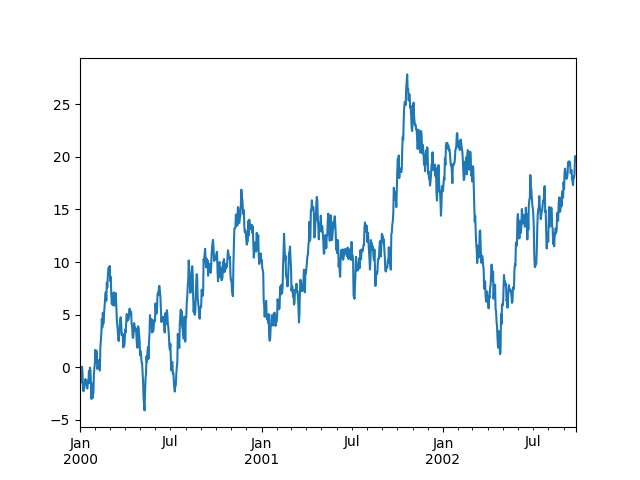
In [69]: ts = md.Series(mt.random.randn(1000),
   ....:                index=md.date_range('1/1/2000', periods=1000))
   ....:

In [70]: ts = ts.cumsum()

In [71]: ts.plot()
Out[71]: <AxesSubplot:>
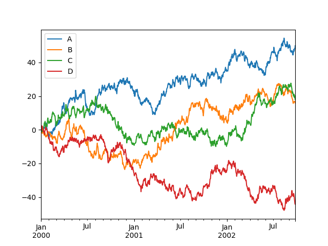
On a DataFrame, the plot() method is a convenience to plot all
of the columns with labels:
In [72]: df = md.DataFrame(mt.random.randn(1000, 4), index=ts.index,
   ....:                   columns=['A', 'B', 'C', 'D'])
   ....:

In [73]: df = df.cumsum()

In [74]: plt.figure()
Out[74]: <Figure size 640x480 with 0 Axes>

In [75]: df.plot()
Out[75]: <AxesSubplot:>

In [76]: plt.legend(loc='best')
Out[76]: <matplotlib.legend.Legend at 0x7efb78dcf490>
Getting data in/out
CSV
In [77]: df.to_csv('foo.csv').execute()
Out[77]:
Empty DataFrame
Columns: []
Index: []
In [78]: md.read_csv('foo.csv').execute()
Out[78]:
     Unnamed: 0          A          B          C          D
0    2000-01-01   0.016940  -1.604006   1.668928  -0.060186
1    2000-01-02   0.692989  -1.548461   1.255053  -0.416344
2    2000-01-03  -0.203780   0.019469  -0.357596   1.403616
3    2000-01-04  -0.035630   0.387176  -0.738632   2.335048
4    2000-01-05  -0.448735  -0.333134  -0.416332   1.687239
..          ...        ...        ...        ...        ...
995  2002-09-22  46.814795  16.743822  19.311003 -39.727366
996  2002-09-23  48.072650  16.531558  20.390472 -41.265423
997  2002-09-24  48.297926  16.877596  19.535501 -42.447506
998  2002-09-25  48.222697  16.829244  19.045099 -43.906503
999  2002-09-26  49.978712  15.924863  17.985864 -44.242937

[1000 rows x 5 columns]