10 minutes to Mars DataFrame#
This is a short introduction to Mars DataFrame which is originated from 10 minutes to pandas.
Customarily, we import as follows:
In [1]: import mars

In [2]: import mars.tensor as mt

In [3]: import mars.dataframe as md
Now create a new default session.
In [4]: mars.new_session()
Out[4]: <mars.deploy.oscar.session.SyncSession at 0x7f480d9aa090>
Object creation#
Creating a Series by passing a list of values, letting it create
a default integer index:
In [5]: s = md.Series([1, 3, 5, mt.nan, 6, 8])

In [6]: s.execute()
Out[6]:
0    1.0
1    3.0
2    5.0
3    NaN
4    6.0
5    8.0
dtype: float64
Creating a DataFrame by passing a Mars tensor, with a datetime index
and labeled columns:
In [7]: dates = md.date_range('20130101', periods=6)

In [8]: dates.execute()
Out[8]:
DatetimeIndex(['2013-01-01', '2013-01-02', '2013-01-03', '2013-01-04',
               '2013-01-05', '2013-01-06'],
              dtype='datetime64[ns]', freq='D')

In [9]: df = md.DataFrame(mt.random.randn(6, 4), index=dates, columns=list('ABCD'))

In [10]: df.execute()
Out[10]:
                   A         B         C         D
2013-01-01  1.301006  1.015965 -1.111896 -1.066854
2013-01-02  1.966591 -1.249476 -1.373745  0.205893
2013-01-03 -0.458425  0.935811 -0.120990  1.452803
2013-01-04 -0.053453  0.558597  0.947676 -1.298274
2013-01-05 -0.796711 -1.477857  2.683626 -0.705510
2013-01-06  0.377050  0.857864  0.362879  0.627550
Creating a DataFrame by passing a dict of objects that can be converted to series-like.
In [11]: df2 = md.DataFrame({'A': 1.,
   ....:                     'B': md.Timestamp('20130102'),
   ....:                     'C': md.Series(1, index=list(range(4)), dtype='float32'),
   ....:                     'D': mt.array([3] * 4, dtype='int32'),
   ....:                     'E': 'foo'})
   ....:

In [12]: df2.execute()
Out[12]:
     A          B    C  D    E
0  1.0 2013-01-02  1.0  3  foo
1  1.0 2013-01-02  1.0  3  foo
2  1.0 2013-01-02  1.0  3  foo
3  1.0 2013-01-02  1.0  3  foo
The columns of the resulting DataFrame have different dtypes.
In [13]: df2.dtypes
Out[13]:
A           float64
B    datetime64[ns]
C           float32
D             int32
E            object
dtype: object
Viewing data#
Here is how to view the top and bottom rows of the frame:
In [14]: df.head().execute()
Out[14]:
                   A         B         C         D
2013-01-01  1.301006  1.015965 -1.111896 -1.066854
2013-01-02  1.966591 -1.249476 -1.373745  0.205893
2013-01-03 -0.458425  0.935811 -0.120990  1.452803
2013-01-04 -0.053453  0.558597  0.947676 -1.298274
2013-01-05 -0.796711 -1.477857  2.683626 -0.705510

In [15]: df.tail(3).execute()
Out[15]:
                   A         B         C         D
2013-01-04 -0.053453  0.558597  0.947676 -1.298274
2013-01-05 -0.796711 -1.477857  2.683626 -0.705510
2013-01-06  0.377050  0.857864  0.362879  0.627550
Display the index, columns:
In [16]: df.index.execute()
Out[16]:
DatetimeIndex(['2013-01-01', '2013-01-02', '2013-01-03', '2013-01-04',
               '2013-01-05', '2013-01-06'],
              dtype='datetime64[ns]', freq='D')

In [17]: df.columns.execute()
Out[17]: Index(['A', 'B', 'C', 'D'], dtype='object')
DataFrame.to_tensor() gives a Mars tensor representation of the underlying data.
Note that this can be an expensive operation when your DataFrame has
columns with different data types, which comes down to a fundamental difference
between DataFrame and tensor: tensors have one dtype for the entire tensor,
while DataFrames have one dtype per column. When you call
DataFrame.to_tensor(), Mars DataFrame will find the tensor dtype that can hold all
of the dtypes in the DataFrame. This may end up being object, which requires
casting every value to a Python object.
For df, our DataFrame of all floating-point values,
DataFrame.to_tensor() is fast and doesn’t require copying data.
In [18]: df.to_tensor().execute()
Out[18]:
array([[ 1.30100623,  1.0159649 , -1.111896  , -1.06685408],
       [ 1.96659072, -1.24947564, -1.3737454 ,  0.20589297],
       [-0.45842486,  0.93581082, -0.12099009,  1.45280267],
       [-0.05345327,  0.55859705,  0.94767623, -1.29827372],
       [-0.79671051, -1.47785669,  2.68362625, -0.70551045],
       [ 0.37704991,  0.85786417,  0.36287932,  0.62755022]])
For df2, the DataFrame with multiple dtypes,
DataFrame.to_tensor() is relatively expensive.
In [19]: df2.to_tensor().execute()
Out[19]:
array([[1.0, Timestamp('2013-01-02 00:00:00'), 1.0, 3, 'foo'],
       [1.0, Timestamp('2013-01-02 00:00:00'), 1.0, 3, 'foo'],
       [1.0, Timestamp('2013-01-02 00:00:00'), 1.0, 3, 'foo'],
       [1.0, Timestamp('2013-01-02 00:00:00'), 1.0, 3, 'foo']],
      dtype=object)
Note
DataFrame.to_tensor() does not include the index or column
labels in the output.
describe() shows a quick statistic summary of your data:
In [20]: df.describe().execute()
Out[20]:
              A         B         C         D
count  6.000000  6.000000  6.000000  6.000000
mean   0.389343  0.106817  0.231258 -0.130732
std    1.062120  1.151753  1.486531  1.073847
min   -0.796711 -1.477857 -1.373745 -1.298274
25%   -0.357182 -0.797457 -0.864170 -0.976518
50%    0.161798  0.708231  0.120945 -0.249809
75%    1.070017  0.916324  0.801477  0.522136
max    1.966591  1.015965  2.683626  1.452803
Sorting by an axis:
In [21]: df.sort_index(axis=1, ascending=False).execute()
Out[21]:
                   D         C         B         A
2013-01-01 -1.066854 -1.111896  1.015965  1.301006
2013-01-02  0.205893 -1.373745 -1.249476  1.966591
2013-01-03  1.452803 -0.120990  0.935811 -0.458425
2013-01-04 -1.298274  0.947676  0.558597 -0.053453
2013-01-05 -0.705510  2.683626 -1.477857 -0.796711
2013-01-06  0.627550  0.362879  0.857864  0.377050
Sorting by values:
In [22]: df.sort_values(by='B').execute()
Out[22]:
                   A         B         C         D
2013-01-05 -0.796711 -1.477857  2.683626 -0.705510
2013-01-02  1.966591 -1.249476 -1.373745  0.205893
2013-01-04 -0.053453  0.558597  0.947676 -1.298274
2013-01-06  0.377050  0.857864  0.362879  0.627550
2013-01-03 -0.458425  0.935811 -0.120990  1.452803
2013-01-01  1.301006  1.015965 -1.111896 -1.066854
Selection#
Note
While standard Python / Numpy expressions for selecting and setting are
intuitive and come in handy for interactive work, for production code, we
recommend the optimized DataFrame data access methods, .at, .iat,
.loc and .iloc.
Getting#
Selecting a single column, which yields a Series,
equivalent to df.A:
In [23]: df['A'].execute()
Out[23]:
2013-01-01    1.301006
2013-01-02    1.966591
2013-01-03   -0.458425
2013-01-04   -0.053453
2013-01-05   -0.796711
2013-01-06    0.377050
Freq: D, Name: A, dtype: float64
Selecting via [], which slices the rows.
In [24]: df[0:3].execute()
Out[24]:
                   A         B         C         D
2013-01-01  1.301006  1.015965 -1.111896 -1.066854
2013-01-02  1.966591 -1.249476 -1.373745  0.205893
2013-01-03 -0.458425  0.935811 -0.120990  1.452803

In [25]: df['20130102':'20130104'].execute()
Out[25]:
                   A         B         C         D
2013-01-02  1.966591 -1.249476 -1.373745  0.205893
2013-01-03 -0.458425  0.935811 -0.120990  1.452803
2013-01-04 -0.053453  0.558597  0.947676 -1.298274
Selection by label#
For getting a cross section using a label:
In [26]: df.loc['20130101'].execute()
Out[26]:
A    1.301006
B    1.015965
C   -1.111896
D   -1.066854
Name: 2013-01-01 00:00:00, dtype: float64
Selecting on a multi-axis by label:
In [27]: df.loc[:, ['A', 'B']].execute()
Out[27]:
                   A         B
2013-01-01  1.301006  1.015965
2013-01-02  1.966591 -1.249476
2013-01-03 -0.458425  0.935811
2013-01-04 -0.053453  0.558597
2013-01-05 -0.796711 -1.477857
2013-01-06  0.377050  0.857864
Showing label slicing, both endpoints are included:
In [28]: df.loc['20130102':'20130104', ['A', 'B']].execute()
Out[28]:
                   A         B
2013-01-02  1.966591 -1.249476
2013-01-03 -0.458425  0.935811
2013-01-04 -0.053453  0.558597
Reduction in the dimensions of the returned object:
In [29]: df.loc['20130102', ['A', 'B']].execute()
Out[29]:
A    1.966591
B   -1.249476
Name: 2013-01-02 00:00:00, dtype: float64
For getting a scalar value:
In [30]: df.loc['20130101', 'A'].execute()
Out[30]: 1.301006234747742
For getting fast access to a scalar (equivalent to the prior method):
In [31]: df.at['20130101', 'A'].execute()
Out[31]: 1.301006234747742
Selection by position#
Select via the position of the passed integers:
In [32]: df.iloc[3].execute()
Out[32]:
A   -0.053453
B    0.558597
C    0.947676
D   -1.298274
Name: 2013-01-04 00:00:00, dtype: float64
By integer slices, acting similar to numpy/python:
In [33]: df.iloc[3:5, 0:2].execute()
Out[33]:
                   A         B
2013-01-04 -0.053453  0.558597
2013-01-05 -0.796711 -1.477857
By lists of integer position locations, similar to the numpy/python style:
In [34]: df.iloc[[1, 2, 4], [0, 2]].execute()
Out[34]:
                   A         C
2013-01-02  1.966591 -1.373745
2013-01-03 -0.458425 -0.120990
2013-01-05 -0.796711  2.683626
For slicing rows explicitly:
In [35]: df.iloc[1:3, :].execute()
Out[35]:
                   A         B         C         D
2013-01-02  1.966591 -1.249476 -1.373745  0.205893
2013-01-03 -0.458425  0.935811 -0.120990  1.452803
For slicing columns explicitly:
In [36]: df.iloc[:, 1:3].execute()
Out[36]:
                   B         C
2013-01-01  1.015965 -1.111896
2013-01-02 -1.249476 -1.373745
2013-01-03  0.935811 -0.120990
2013-01-04  0.558597  0.947676
2013-01-05 -1.477857  2.683626
2013-01-06  0.857864  0.362879
For getting a value explicitly:
In [37]: df.iloc[1, 1].execute()
Out[37]: -1.249475639706685
For getting fast access to a scalar (equivalent to the prior method):
In [38]: df.iat[1, 1].execute()
Out[38]: -1.249475639706685
Boolean indexing#
Using a single column’s values to select data.
In [39]: df[df['A'] > 0].execute()
Out[39]:
                   A         B         C         D
2013-01-01  1.301006  1.015965 -1.111896 -1.066854
2013-01-02  1.966591 -1.249476 -1.373745  0.205893
2013-01-06  0.377050  0.857864  0.362879  0.627550
Selecting values from a DataFrame where a boolean condition is met.
In [40]: df[df > 0].execute()
Out[40]:
                   A         B         C         D
2013-01-01  1.301006  1.015965       NaN       NaN
2013-01-02  1.966591       NaN       NaN  0.205893
2013-01-03       NaN  0.935811       NaN  1.452803
2013-01-04       NaN  0.558597  0.947676       NaN
2013-01-05       NaN       NaN  2.683626       NaN
2013-01-06  0.377050  0.857864  0.362879  0.627550
Operations#
Stats#
Operations in general exclude missing data.
Performing a descriptive statistic:
In [41]: df.mean().execute()
Out[41]:
A    0.389343
B    0.106817
C    0.231258
D   -0.130732
dtype: float64
Same operation on the other axis:
In [42]: df.mean(1).execute()
Out[42]:
2013-01-01    0.034555
2013-01-02   -0.112684
2013-01-03    0.452300
2013-01-04    0.038637
2013-01-05   -0.074113
2013-01-06    0.556336
Freq: D, dtype: float64
Operating with objects that have different dimensionality and need alignment. In addition, Mars DataFrame automatically broadcasts along the specified dimension.
In [43]: s = md.Series([1, 3, 5, mt.nan, 6, 8], index=dates).shift(2)

In [44]: s.execute()
Out[44]:
2013-01-01    NaN
2013-01-02    NaN
2013-01-03    1.0
2013-01-04    3.0
2013-01-05    5.0
2013-01-06    NaN
Freq: D, dtype: float64

In [45]: df.sub(s, axis='index').execute()
Out[45]:
                   A         B         C         D
2013-01-01       NaN       NaN       NaN       NaN
2013-01-02       NaN       NaN       NaN       NaN
2013-01-03 -1.458425 -0.064189 -1.120990  0.452803
2013-01-04 -3.053453 -2.441403 -2.052324 -4.298274
2013-01-05 -5.796711 -6.477857 -2.316374 -5.705510
2013-01-06       NaN       NaN       NaN       NaN
Apply#
Applying functions to the data:
In [46]: df.apply(lambda x: x.max() - x.min()).execute()
Out[46]:
A    2.763301
B    2.493822
C    4.057372
D    2.751076
dtype: float64
String Methods#
Series is equipped with a set of string processing methods in the str attribute that make it easy to operate on each element of the array, as in the code snippet below. Note that pattern-matching in str generally uses regular expressions by default (and in some cases always uses them). See more at Vectorized String Methods.
In [47]: s = md.Series(['A', 'B', 'C', 'Aaba', 'Baca', mt.nan, 'CABA', 'dog', 'cat'])

In [48]: s.str.lower().execute()
Out[48]:
0       a
1       b
2       c
3    aaba
4    baca
5     NaN
6    caba
7     dog
8     cat
dtype: object
Merge#
Concat#
Mars DataFrame provides various facilities for easily combining together Series and DataFrame objects with various kinds of set logic for the indexes and relational algebra functionality in the case of join / merge-type operations.
Concatenating DataFrame objects together with concat():
In [49]: df = md.DataFrame(mt.random.randn(10, 4))

In [50]: df.execute()
Out[50]:
          0         1         2         3
0  1.602503  0.637887 -1.055659 -0.870901
1 -0.207847  0.578935  0.187930 -0.598496
2  0.248635  0.732671  0.040768  0.086089
3  2.445247 -1.828383  0.319453  0.499161
4  0.002242 -0.532310  0.465981 -0.044516
5 -0.568768 -0.783130 -0.193903  0.527273
6 -0.581460  1.081464 -0.784618  0.985970
7  0.820671 -0.089649 -0.169568  1.136980
8 -1.262083 -0.484230 -0.966078 -0.271765
9  1.484495  0.025214 -0.386365 -0.157642

# break it into pieces
In [51]: pieces = [df[:3], df[3:7], df[7:]]

In [52]: md.concat(pieces).execute()
Out[52]:
          0         1         2         3
0  1.602503  0.637887 -1.055659 -0.870901
1 -0.207847  0.578935  0.187930 -0.598496
2  0.248635  0.732671  0.040768  0.086089
3  2.445247 -1.828383  0.319453  0.499161
4  0.002242 -0.532310  0.465981 -0.044516
5 -0.568768 -0.783130 -0.193903  0.527273
6 -0.581460  1.081464 -0.784618  0.985970
7  0.820671 -0.089649 -0.169568  1.136980
8 -1.262083 -0.484230 -0.966078 -0.271765
9  1.484495  0.025214 -0.386365 -0.157642
Join#
SQL style merges. See the Database style joining section.
In [53]: left = md.DataFrame({'key': ['foo', 'foo'], 'lval': [1, 2]})

In [54]: right = md.DataFrame({'key': ['foo', 'foo'], 'rval': [4, 5]})

In [55]: left.execute()
Out[55]:
   key  lval
0  foo     1
1  foo     2

In [56]: right.execute()
Out[56]:
   key  rval
0  foo     4
1  foo     5

In [57]: md.merge(left, right, on='key').execute()
Out[57]:
   key  lval  rval
0  foo     1     4
1  foo     1     5
2  foo     2     4
3  foo     2     5
Another example that can be given is:
In [58]: left = md.DataFrame({'key': ['foo', 'bar'], 'lval': [1, 2]})

In [59]: right = md.DataFrame({'key': ['foo', 'bar'], 'rval': [4, 5]})

In [60]: left.execute()
Out[60]:
   key  lval
0  foo     1
1  bar     2

In [61]: right.execute()
Out[61]:
   key  rval
0  foo     4
1  bar     5

In [62]: md.merge(left, right, on='key').execute()
Out[62]:
   key  lval  rval
0  foo     1     4
1  bar     2     5
Grouping#
By “group by” we are referring to a process involving one or more of the following steps:
Splitting the data into groups based on some criteria
Applying a function to each group independently
Combining the results into a data structure
In [63]: df = md.DataFrame({'A': ['foo', 'bar', 'foo', 'bar',
   ....:                          'foo', 'bar', 'foo', 'foo'],
   ....:                    'B': ['one', 'one', 'two', 'three',
   ....:                          'two', 'two', 'one', 'three'],
   ....:                    'C': mt.random.randn(8),
   ....:                    'D': mt.random.randn(8)})
   ....:

In [64]: df.execute()
Out[64]:
     A      B         C         D
0  foo    one  0.344229  0.651770
1  bar    one  1.545709  0.283630
2  foo    two -0.284916 -0.134626
3  bar  three  1.233326 -0.380892
4  foo    two -0.279609  1.131483
5  bar    two  0.504077  0.001285
6  foo    one -1.799578  0.772063
7  foo  three  0.397000 -1.274884
Grouping and then applying the sum() function to the resulting
groups.
In [65]: df.groupby('A').sum().execute()
Out[65]:
            C         D
A
bar  3.283112 -0.095977
foo -1.622873  1.145808
Grouping by multiple columns forms a hierarchical index, and again we can apply the sum function.
In [66]: df.groupby(['A', 'B']).sum().execute()
Out[66]:
                  C         D
A   B
bar one    1.545709  0.283630
    three  1.233326 -0.380892
    two    0.504077  0.001285
foo one   -1.455349  1.423834
    three  0.397000 -1.274884
    two   -0.564524  0.996858
Plotting#
We use the standard convention for referencing the matplotlib API:
In [67]: import matplotlib.pyplot as plt

In [68]: plt.close('all')
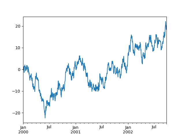
In [69]: ts = md.Series(mt.random.randn(1000),
   ....:                index=md.date_range('1/1/2000', periods=1000))
   ....:

In [70]: ts = ts.cumsum()

In [71]: ts.plot()
Out[71]: <AxesSubplot:>
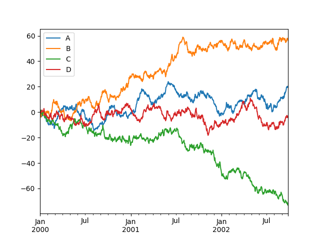
On a DataFrame, the plot() method is a convenience to plot all
of the columns with labels:
In [72]: df = md.DataFrame(mt.random.randn(1000, 4), index=ts.index,
   ....:                   columns=['A', 'B', 'C', 'D'])
   ....:

In [73]: df = df.cumsum()

In [74]: plt.figure()
Out[74]: <Figure size 640x480 with 0 Axes>

In [75]: df.plot()
Out[75]: <AxesSubplot:>

In [76]: plt.legend(loc='best')
Out[76]: <matplotlib.legend.Legend at 0x7f480dbb5190>
Getting data in/out#
CSV#
In [77]: df.to_csv('foo.csv').execute()
Out[77]:
Empty DataFrame
Columns: []
Index: []
In [78]: md.read_csv('foo.csv').execute()
Out[78]:
     Unnamed: 0          A          B          C         D
0    2000-01-01   0.701958  -0.473432   0.091628  0.611637
1    2000-01-02  -0.802138  -1.265910   1.449300 -0.170869
2    2000-01-03  -0.922035  -2.449515   1.584012 -0.655200
3    2000-01-04  -0.308032  -3.807212   1.448196  0.218207
4    2000-01-05  -1.003870  -3.894358   1.401089  0.039483
..          ...        ...        ...        ...       ...
995  2002-09-22  19.508035  56.998958 -70.809038 -2.759202
996  2002-09-23  20.269463  58.095389 -71.245478 -2.915498
997  2002-09-24  19.340480  57.421578 -72.614199 -4.340794
998  2002-09-25  19.637776  56.936608 -71.965457 -3.360895
999  2002-09-26  20.149852  56.302042 -73.130355 -3.954408

[1000 rows x 5 columns]