mars.dataframe.Series.plot.density#
- Series.plot.density(*args, **kwargs)#
Generate Kernel Density Estimate plot using Gaussian kernels.
In statistics, kernel density estimation (KDE) is a non-parametric way to estimate the probability density function (PDF) of a random variable. This function uses Gaussian kernels and includes automatic bandwidth determination.
- Parameters
bw_method (str, scalar or callable, optional) – The method used to calculate the estimator bandwidth. This can be ‘scott’, ‘silverman’, a scalar constant or a callable. If None (default), ‘scott’ is used. See
scipy.stats.gaussian_kdefor more information.ind (NumPy array or int, optional) – Evaluation points for the estimated PDF. If None (default), 1000 equally spaced points are used. If ind is a NumPy array, the KDE is evaluated at the points passed. If ind is an integer, ind number of equally spaced points are used.
**kwargs – Additional keyword arguments are documented in
pandas.%(this-datatype)s.plot().
- Return type
matplotlib.axes.Axes or numpy.ndarray of them
See also
scipy.stats.gaussian_kdeRepresentation of a kernel-density estimate using Gaussian kernels. This is the function used internally to estimate the PDF.
Examples
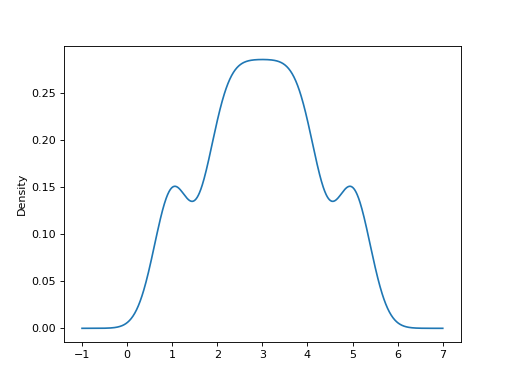
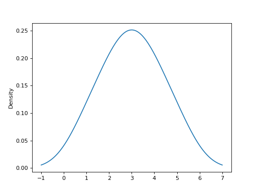
Given a Series of points randomly sampled from an unknown distribution, estimate its PDF using KDE with automatic bandwidth determination and plot the results, evaluating them at 1000 equally spaced points (default):
(Source code, png, hires.png, pdf)

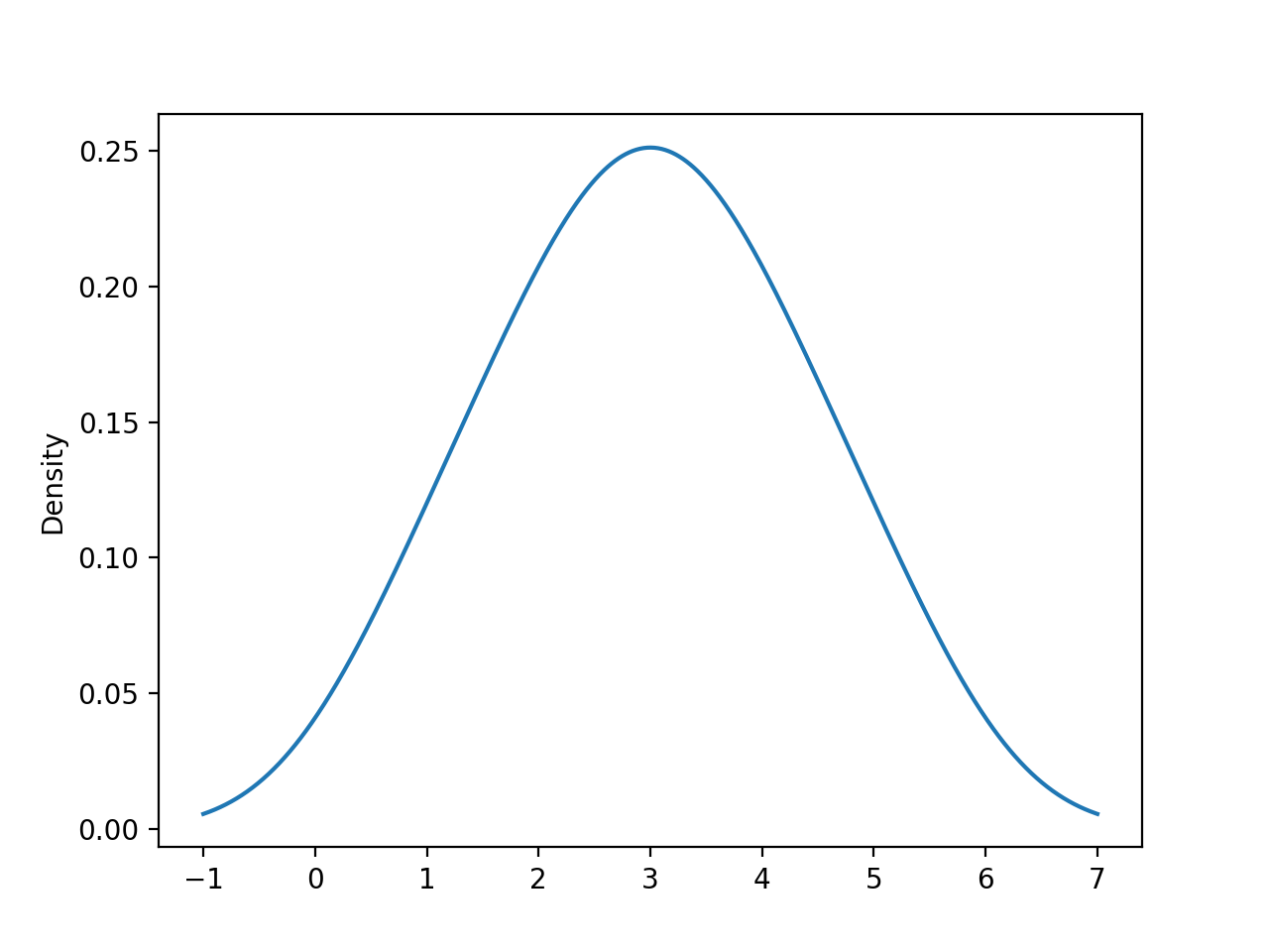
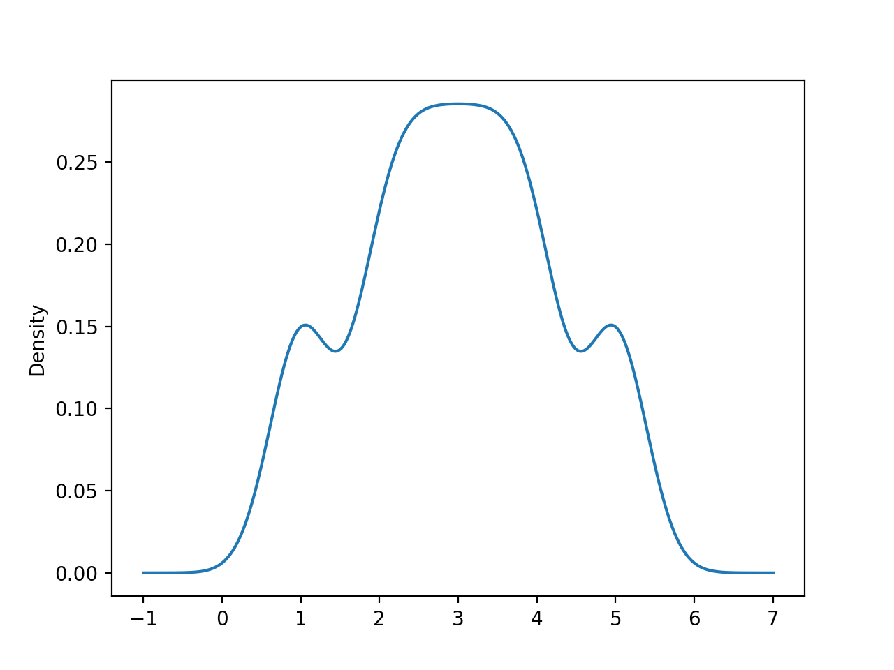
A scalar bandwidth can be specified. Using a small bandwidth value can lead to over-fitting, while using a large bandwidth value may result in under-fitting:
(Source code, png, hires.png, pdf)
(Source code, png, hires.png, pdf)

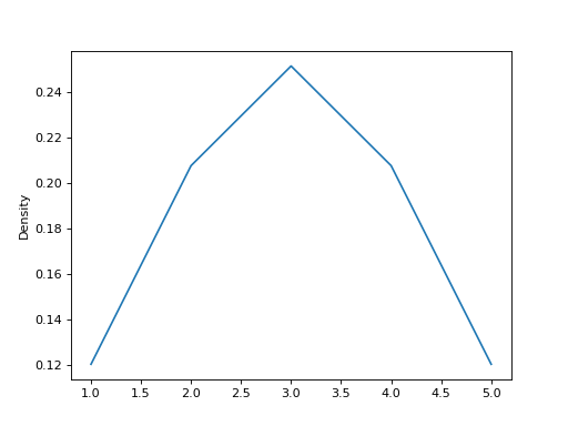
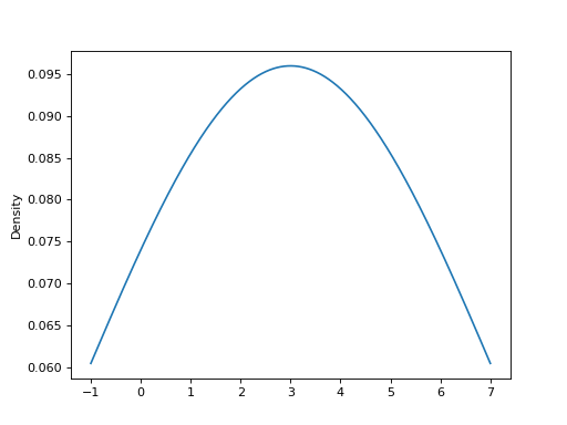
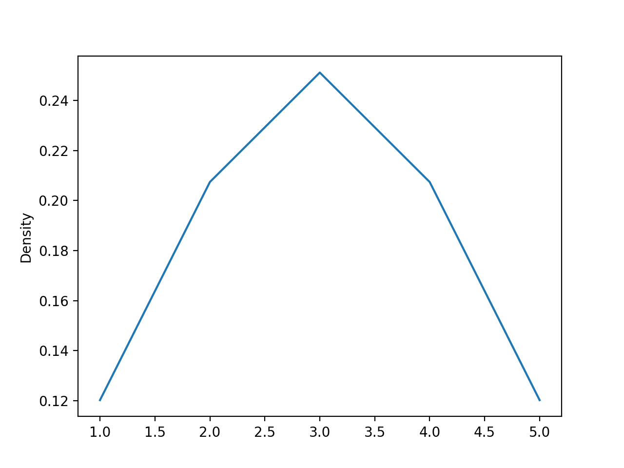
Finally, the ind parameter determines the evaluation points for the plot of the estimated PDF:
(Source code, png, hires.png, pdf)
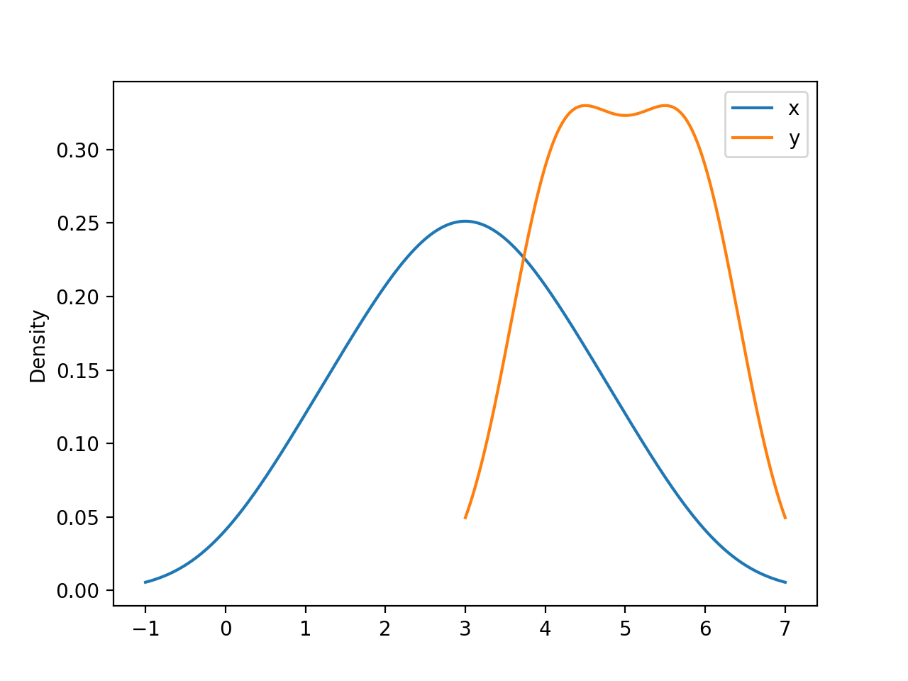
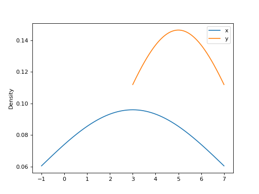
For DataFrame, it works in the same way:
(Source code, png, hires.png, pdf)
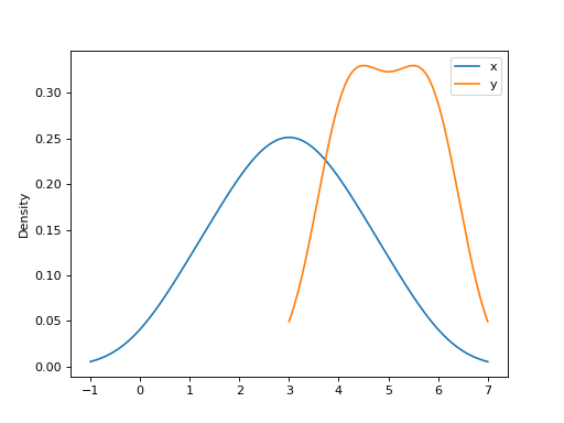
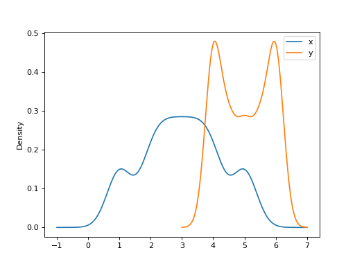
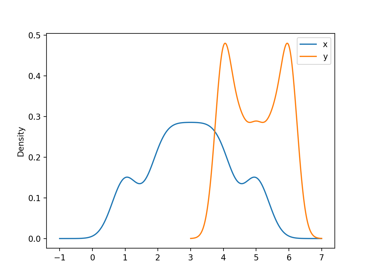
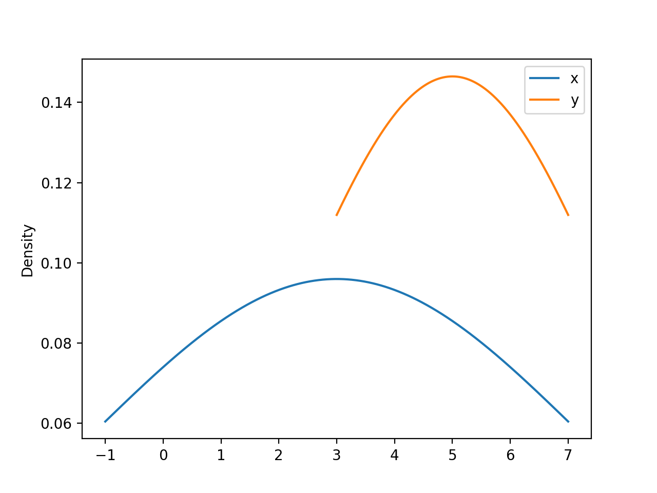
A scalar bandwidth can be specified. Using a small bandwidth value can lead to over-fitting, while using a large bandwidth value may result in under-fitting:
(Source code, png, hires.png, pdf)

(Source code, png, hires.png, pdf)

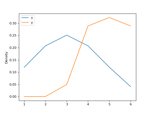
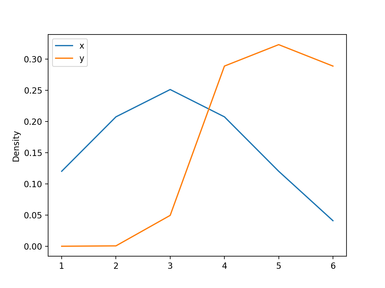
Finally, the ind parameter determines the evaluation points for the plot of the estimated PDF:
(Source code, png, hires.png, pdf)