10 minutes to Mars DataFrame#
This is a short introduction to Mars DataFrame which is originated from 10 minutes to pandas.
Customarily, we import as follows:
In [1]: import mars

In [2]: import mars.tensor as mt

In [3]: import mars.dataframe as md
Now create a new default session.
In [4]: mars.new_session()
Out[4]: <mars.deploy.oscar.session.SyncSession at 0x7f9f730edf10>
Object creation#
Creating a Series by passing a list of values, letting it create
a default integer index:
In [5]: s = md.Series([1, 3, 5, mt.nan, 6, 8])

In [6]: s.execute()
Out[6]:
0    1.0
1    3.0
2    5.0
3    NaN
4    6.0
5    8.0
dtype: float64
Creating a DataFrame by passing a Mars tensor, with a datetime index
and labeled columns:
In [7]: dates = md.date_range('20130101', periods=6)

In [8]: dates.execute()
Out[8]:
DatetimeIndex(['2013-01-01', '2013-01-02', '2013-01-03', '2013-01-04',
               '2013-01-05', '2013-01-06'],
              dtype='datetime64[ns]', freq='D')

In [9]: df = md.DataFrame(mt.random.randn(6, 4), index=dates, columns=list('ABCD'))

In [10]: df.execute()
Out[10]:
                   A         B         C         D
2013-01-01 -0.234470 -1.674278  0.754438 -0.791787
2013-01-02  0.786225  1.931285 -1.424769 -0.788837
2013-01-03  0.143058 -0.127653 -0.005265 -1.341106
2013-01-04  0.757987  0.329978  0.332887 -0.151451
2013-01-05 -0.173489 -1.656515 -0.816907  0.428194
2013-01-06  0.928163  0.683618  1.102615 -1.992196
Creating a DataFrame by passing a dict of objects that can be converted to series-like.
In [11]: df2 = md.DataFrame({'A': 1.,
   ....:                     'B': md.Timestamp('20130102'),
   ....:                     'C': md.Series(1, index=list(range(4)), dtype='float32'),
   ....:                     'D': mt.array([3] * 4, dtype='int32'),
   ....:                     'E': 'foo'})
   ....:

In [12]: df2.execute()
Out[12]:
     A          B    C  D    E
0  1.0 2013-01-02  1.0  3  foo
1  1.0 2013-01-02  1.0  3  foo
2  1.0 2013-01-02  1.0  3  foo
3  1.0 2013-01-02  1.0  3  foo
The columns of the resulting DataFrame have different dtypes.
In [13]: df2.dtypes
Out[13]:
A           float64
B    datetime64[ns]
C           float32
D             int32
E            object
dtype: object
Viewing data#
Here is how to view the top and bottom rows of the frame:
In [14]: df.head().execute()
Out[14]:
                   A         B         C         D
2013-01-01 -0.234470 -1.674278  0.754438 -0.791787
2013-01-02  0.786225  1.931285 -1.424769 -0.788837
2013-01-03  0.143058 -0.127653 -0.005265 -1.341106
2013-01-04  0.757987  0.329978  0.332887 -0.151451
2013-01-05 -0.173489 -1.656515 -0.816907  0.428194

In [15]: df.tail(3).execute()
Out[15]:
                   A         B         C         D
2013-01-04  0.757987  0.329978  0.332887 -0.151451
2013-01-05 -0.173489 -1.656515 -0.816907  0.428194
2013-01-06  0.928163  0.683618  1.102615 -1.992196
Display the index, columns:
In [16]: df.index.execute()
Out[16]:
DatetimeIndex(['2013-01-01', '2013-01-02', '2013-01-03', '2013-01-04',
               '2013-01-05', '2013-01-06'],
              dtype='datetime64[ns]', freq='D')

In [17]: df.columns.execute()
Out[17]: Index(['A', 'B', 'C', 'D'], dtype='object')
DataFrame.to_tensor() gives a Mars tensor representation of the underlying data.
Note that this can be an expensive operation when your DataFrame has
columns with different data types, which comes down to a fundamental difference
between DataFrame and tensor: tensors have one dtype for the entire tensor,
while DataFrames have one dtype per column. When you call
DataFrame.to_tensor(), Mars DataFrame will find the tensor dtype that can hold all
of the dtypes in the DataFrame. This may end up being object, which requires
casting every value to a Python object.
For df, our DataFrame of all floating-point values,
DataFrame.to_tensor() is fast and doesn’t require copying data.
In [18]: df.to_tensor().execute()
Out[18]:
array([[-0.23447019, -1.67427838,  0.7544377 , -0.79178729],
       [ 0.7862249 ,  1.93128531, -1.42476909, -0.78883699],
       [ 0.14305808, -0.12765314, -0.00526497, -1.34110595],
       [ 0.75798733,  0.3299783 ,  0.33288706, -0.15145094],
       [-0.1734895 , -1.65651467, -0.81690741,  0.42819413],
       [ 0.92816277,  0.68361823,  1.10261483, -1.99219597]])
For df2, the DataFrame with multiple dtypes,
DataFrame.to_tensor() is relatively expensive.
In [19]: df2.to_tensor().execute()
Out[19]:
array([[1.0, Timestamp('2013-01-02 00:00:00'), 1.0, 3, 'foo'],
       [1.0, Timestamp('2013-01-02 00:00:00'), 1.0, 3, 'foo'],
       [1.0, Timestamp('2013-01-02 00:00:00'), 1.0, 3, 'foo'],
       [1.0, Timestamp('2013-01-02 00:00:00'), 1.0, 3, 'foo']],
      dtype=object)
Note
DataFrame.to_tensor() does not include the index or column
labels in the output.
describe() shows a quick statistic summary of your data:
In [20]: df.describe().execute()
Out[20]:
              A         B         C         D
count  6.000000  6.000000  6.000000  6.000000
mean   0.367912 -0.085594 -0.009500 -0.772864
std    0.519146  1.401832  0.958388  0.853109
min   -0.234470 -1.674278 -1.424769 -1.992196
25%   -0.094353 -1.274299 -0.613997 -1.203776
50%    0.450523  0.101163  0.163811 -0.790312
75%    0.779166  0.595208  0.649050 -0.310797
max    0.928163  1.931285  1.102615  0.428194
Sorting by an axis:
In [21]: df.sort_index(axis=1, ascending=False).execute()
Out[21]:
                   D         C         B         A
2013-01-01 -0.791787  0.754438 -1.674278 -0.234470
2013-01-02 -0.788837 -1.424769  1.931285  0.786225
2013-01-03 -1.341106 -0.005265 -0.127653  0.143058
2013-01-04 -0.151451  0.332887  0.329978  0.757987
2013-01-05  0.428194 -0.816907 -1.656515 -0.173489
2013-01-06 -1.992196  1.102615  0.683618  0.928163
Sorting by values:
In [22]: df.sort_values(by='B').execute()
Out[22]:
                   A         B         C         D
2013-01-01 -0.234470 -1.674278  0.754438 -0.791787
2013-01-05 -0.173489 -1.656515 -0.816907  0.428194
2013-01-03  0.143058 -0.127653 -0.005265 -1.341106
2013-01-04  0.757987  0.329978  0.332887 -0.151451
2013-01-06  0.928163  0.683618  1.102615 -1.992196
2013-01-02  0.786225  1.931285 -1.424769 -0.788837
Selection#
Note
While standard Python / Numpy expressions for selecting and setting are
intuitive and come in handy for interactive work, for production code, we
recommend the optimized DataFrame data access methods, .at, .iat,
.loc and .iloc.
Getting#
Selecting a single column, which yields a Series,
equivalent to df.A:
In [23]: df['A'].execute()
Out[23]:
2013-01-01   -0.234470
2013-01-02    0.786225
2013-01-03    0.143058
2013-01-04    0.757987
2013-01-05   -0.173489
2013-01-06    0.928163
Freq: D, Name: A, dtype: float64
Selecting via [], which slices the rows.
In [24]: df[0:3].execute()
Out[24]:
                   A         B         C         D
2013-01-01 -0.234470 -1.674278  0.754438 -0.791787
2013-01-02  0.786225  1.931285 -1.424769 -0.788837
2013-01-03  0.143058 -0.127653 -0.005265 -1.341106

In [25]: df['20130102':'20130104'].execute()
Out[25]:
                   A         B         C         D
2013-01-02  0.786225  1.931285 -1.424769 -0.788837
2013-01-03  0.143058 -0.127653 -0.005265 -1.341106
2013-01-04  0.757987  0.329978  0.332887 -0.151451
Selection by label#
For getting a cross section using a label:
In [26]: df.loc['20130101'].execute()
Out[26]:
A   -0.234470
B   -1.674278
C    0.754438
D   -0.791787
Name: 2013-01-01 00:00:00, dtype: float64
Selecting on a multi-axis by label:
In [27]: df.loc[:, ['A', 'B']].execute()
Out[27]:
                   A         B
2013-01-01 -0.234470 -1.674278
2013-01-02  0.786225  1.931285
2013-01-03  0.143058 -0.127653
2013-01-04  0.757987  0.329978
2013-01-05 -0.173489 -1.656515
2013-01-06  0.928163  0.683618
Showing label slicing, both endpoints are included:
In [28]: df.loc['20130102':'20130104', ['A', 'B']].execute()
Out[28]:
                   A         B
2013-01-02  0.786225  1.931285
2013-01-03  0.143058 -0.127653
2013-01-04  0.757987  0.329978
Reduction in the dimensions of the returned object:
In [29]: df.loc['20130102', ['A', 'B']].execute()
Out[29]:
A    0.786225
B    1.931285
Name: 2013-01-02 00:00:00, dtype: float64
For getting a scalar value:
In [30]: df.loc['20130101', 'A'].execute()
Out[30]: -0.2344701945616982
For getting fast access to a scalar (equivalent to the prior method):
In [31]: df.at['20130101', 'A'].execute()
Out[31]: -0.2344701945616982
Selection by position#
Select via the position of the passed integers:
In [32]: df.iloc[3].execute()
Out[32]:
A    0.757987
B    0.329978
C    0.332887
D   -0.151451
Name: 2013-01-04 00:00:00, dtype: float64
By integer slices, acting similar to numpy/python:
In [33]: df.iloc[3:5, 0:2].execute()
Out[33]:
                   A         B
2013-01-04  0.757987  0.329978
2013-01-05 -0.173489 -1.656515
By lists of integer position locations, similar to the numpy/python style:
In [34]: df.iloc[[1, 2, 4], [0, 2]].execute()
Out[34]:
                   A         C
2013-01-02  0.786225 -1.424769
2013-01-03  0.143058 -0.005265
2013-01-05 -0.173489 -0.816907
For slicing rows explicitly:
In [35]: df.iloc[1:3, :].execute()
Out[35]:
                   A         B         C         D
2013-01-02  0.786225  1.931285 -1.424769 -0.788837
2013-01-03  0.143058 -0.127653 -0.005265 -1.341106
For slicing columns explicitly:
In [36]: df.iloc[:, 1:3].execute()
Out[36]:
                   B         C
2013-01-01 -1.674278  0.754438
2013-01-02  1.931285 -1.424769
2013-01-03 -0.127653 -0.005265
2013-01-04  0.329978  0.332887
2013-01-05 -1.656515 -0.816907
2013-01-06  0.683618  1.102615
For getting a value explicitly:
In [37]: df.iloc[1, 1].execute()
Out[37]: 1.9312853057474288
For getting fast access to a scalar (equivalent to the prior method):
In [38]: df.iat[1, 1].execute()
Out[38]: 1.9312853057474288
Boolean indexing#
Using a single column’s values to select data.
In [39]: df[df['A'] > 0].execute()
Out[39]:
                   A         B         C         D
2013-01-02  0.786225  1.931285 -1.424769 -0.788837
2013-01-03  0.143058 -0.127653 -0.005265 -1.341106
2013-01-04  0.757987  0.329978  0.332887 -0.151451
2013-01-06  0.928163  0.683618  1.102615 -1.992196
Selecting values from a DataFrame where a boolean condition is met.
In [40]: df[df > 0].execute()
Out[40]:
                   A         B         C         D
2013-01-01       NaN       NaN  0.754438       NaN
2013-01-02  0.786225  1.931285       NaN       NaN
2013-01-03  0.143058       NaN       NaN       NaN
2013-01-04  0.757987  0.329978  0.332887       NaN
2013-01-05       NaN       NaN       NaN  0.428194
2013-01-06  0.928163  0.683618  1.102615       NaN
Operations#
Stats#
Operations in general exclude missing data.
Performing a descriptive statistic:
In [41]: df.mean().execute()
Out[41]:
A    0.367912
B   -0.085594
C   -0.009500
D   -0.772864
dtype: float64
Same operation on the other axis:
In [42]: df.mean(1).execute()
Out[42]:
2013-01-01   -0.486525
2013-01-02    0.125976
2013-01-03   -0.332741
2013-01-04    0.317350
2013-01-05   -0.554679
2013-01-06    0.180550
Freq: D, dtype: float64
Operating with objects that have different dimensionality and need alignment. In addition, Mars DataFrame automatically broadcasts along the specified dimension.
In [43]: s = md.Series([1, 3, 5, mt.nan, 6, 8], index=dates).shift(2)

In [44]: s.execute()
Out[44]:
2013-01-01    NaN
2013-01-02    NaN
2013-01-03    1.0
2013-01-04    3.0
2013-01-05    5.0
2013-01-06    NaN
Freq: D, dtype: float64

In [45]: df.sub(s, axis='index').execute()
Out[45]:
                   A         B         C         D
2013-01-01       NaN       NaN       NaN       NaN
2013-01-02       NaN       NaN       NaN       NaN
2013-01-03 -0.856942 -1.127653 -1.005265 -2.341106
2013-01-04 -2.242013 -2.670022 -2.667113 -3.151451
2013-01-05 -5.173489 -6.656515 -5.816907 -4.571806
2013-01-06       NaN       NaN       NaN       NaN
Apply#
Applying functions to the data:
In [46]: df.apply(lambda x: x.max() - x.min()).execute()
Out[46]:
A    1.162633
B    3.605564
C    2.527384
D    2.420390
dtype: float64
String Methods#
Series is equipped with a set of string processing methods in the str attribute that make it easy to operate on each element of the array, as in the code snippet below. Note that pattern-matching in str generally uses regular expressions by default (and in some cases always uses them). See more at Vectorized String Methods.
In [47]: s = md.Series(['A', 'B', 'C', 'Aaba', 'Baca', mt.nan, 'CABA', 'dog', 'cat'])

In [48]: s.str.lower().execute()
Out[48]:
0       a
1       b
2       c
3    aaba
4    baca
5     NaN
6    caba
7     dog
8     cat
dtype: object
Merge#
Concat#
Mars DataFrame provides various facilities for easily combining together Series and DataFrame objects with various kinds of set logic for the indexes and relational algebra functionality in the case of join / merge-type operations.
Concatenating DataFrame objects together with concat():
In [49]: df = md.DataFrame(mt.random.randn(10, 4))

In [50]: df.execute()
Out[50]:
          0         1         2         3
0  0.192324 -0.627652  0.244818 -0.173757
1 -0.622024 -0.712650  0.477553  0.595258
2  0.660431  0.822757  0.959371 -0.328558
3  0.465535  0.369663 -0.773703 -0.356157
4  1.331941 -0.330811 -0.170924 -1.449218
5 -1.156350 -2.799176  0.626655 -0.897829
6  0.589205  1.087337 -0.020651 -1.026555
7  1.125569 -0.103166  0.643546  1.097255
8 -0.788393  1.017578 -1.207668  0.014432
9  1.385419  0.397382  0.340151 -0.188651

# break it into pieces
In [51]: pieces = [df[:3], df[3:7], df[7:]]

In [52]: md.concat(pieces).execute()
Out[52]:
          0         1         2         3
0  0.192324 -0.627652  0.244818 -0.173757
1 -0.622024 -0.712650  0.477553  0.595258
2  0.660431  0.822757  0.959371 -0.328558
3  0.465535  0.369663 -0.773703 -0.356157
4  1.331941 -0.330811 -0.170924 -1.449218
5 -1.156350 -2.799176  0.626655 -0.897829
6  0.589205  1.087337 -0.020651 -1.026555
7  1.125569 -0.103166  0.643546  1.097255
8 -0.788393  1.017578 -1.207668  0.014432
9  1.385419  0.397382  0.340151 -0.188651
Join#
SQL style merges. See the Database style joining section.
In [53]: left = md.DataFrame({'key': ['foo', 'foo'], 'lval': [1, 2]})

In [54]: right = md.DataFrame({'key': ['foo', 'foo'], 'rval': [4, 5]})

In [55]: left.execute()
Out[55]:
   key  lval
0  foo     1
1  foo     2

In [56]: right.execute()
Out[56]:
   key  rval
0  foo     4
1  foo     5

In [57]: md.merge(left, right, on='key').execute()
Out[57]:
   key  lval  rval
0  foo     1     4
1  foo     1     5
2  foo     2     4
3  foo     2     5
Another example that can be given is:
In [58]: left = md.DataFrame({'key': ['foo', 'bar'], 'lval': [1, 2]})

In [59]: right = md.DataFrame({'key': ['foo', 'bar'], 'rval': [4, 5]})

In [60]: left.execute()
Out[60]:
   key  lval
0  foo     1
1  bar     2

In [61]: right.execute()
Out[61]:
   key  rval
0  foo     4
1  bar     5

In [62]: md.merge(left, right, on='key').execute()
Out[62]:
   key  lval  rval
0  foo     1     4
1  bar     2     5
Grouping#
By “group by” we are referring to a process involving one or more of the following steps:
Splitting the data into groups based on some criteria
Applying a function to each group independently
Combining the results into a data structure
In [63]: df = md.DataFrame({'A': ['foo', 'bar', 'foo', 'bar',
   ....:                          'foo', 'bar', 'foo', 'foo'],
   ....:                    'B': ['one', 'one', 'two', 'three',
   ....:                          'two', 'two', 'one', 'three'],
   ....:                    'C': mt.random.randn(8),
   ....:                    'D': mt.random.randn(8)})
   ....:

In [64]: df.execute()
Out[64]:
     A      B         C         D
0  foo    one  0.172833 -0.590667
1  bar    one -1.570249 -0.259594
2  foo    two  1.619853 -2.118202
3  bar  three -0.148262 -0.451868
4  foo    two -0.300233  0.035199
5  bar    two  1.536751  0.300277
6  foo    one -0.420759  0.689130
7  foo  three -0.603313 -0.241116
Grouping and then applying the sum() function to the resulting
groups.
In [65]: df.groupby('A').sum().execute()
Out[65]:
            C         D
A
bar -0.181760 -0.411185
foo  0.468382 -2.225655
Grouping by multiple columns forms a hierarchical index, and again we can apply the sum function.
In [66]: df.groupby(['A', 'B']).sum().execute()
Out[66]:
                  C         D
A   B
bar one   -1.570249 -0.259594
    three -0.148262 -0.451868
    two    1.536751  0.300277
foo one   -0.247926  0.098463
    three -0.603313 -0.241116
    two    1.319620 -2.083003
Plotting#
We use the standard convention for referencing the matplotlib API:
In [67]: import matplotlib.pyplot as plt

In [68]: plt.close('all')
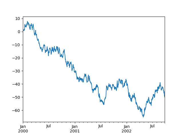
In [69]: ts = md.Series(mt.random.randn(1000),
   ....:                index=md.date_range('1/1/2000', periods=1000))
   ....:

In [70]: ts = ts.cumsum()

In [71]: ts.plot()
Out[71]: <AxesSubplot:>
On a DataFrame, the plot() method is a convenience to plot all
of the columns with labels:
In [72]: df = md.DataFrame(mt.random.randn(1000, 4), index=ts.index,
   ....:                   columns=['A', 'B', 'C', 'D'])
   ....:

In [73]: df = df.cumsum()

In [74]: plt.figure()
Out[74]: <Figure size 640x480 with 0 Axes>

In [75]: df.plot()
Out[75]: <AxesSubplot:>

In [76]: plt.legend(loc='best')
Out[76]: <matplotlib.legend.Legend at 0x7f9f76b8d790>

Getting data in/out#
CSV#
In [77]: df.to_csv('foo.csv').execute()
Out[77]:
Empty DataFrame
Columns: []
Index: []
In [78]: md.read_csv('foo.csv').execute()
Out[78]:
     Unnamed: 0          A          B         C          D
0    2000-01-01   1.120135  -1.031429 -0.668207   0.112060
1    2000-01-02   0.371544  -1.434101 -2.407958  -0.848452
2    2000-01-03   1.096145  -1.824855 -3.521793  -1.907277
3    2000-01-04   1.143595  -2.779346 -2.975172  -0.289020
4    2000-01-05   2.162817  -4.663960 -3.130795  -0.386988
..          ...        ...        ...       ...        ...
995  2002-09-22 -60.874924  33.566216 -7.820672  42.251204
996  2002-09-23 -62.079016  32.353687 -6.318389  42.945471
997  2002-09-24 -63.284392  33.583824 -4.909498  42.905871
998  2002-09-25 -64.254273  34.038688 -5.296638  42.836426
999  2002-09-26 -63.254049  34.244112 -4.727660  40.845142

[1000 rows x 5 columns]